Persuasion with Verifiable Information

Abstract

1. Introduction

Persuasion with verifiable information plays an essential role in many economic settings, including courtrooms, electoral campaigns, product advertising, financial disclosure, and job market signaling. In a courtroom, a prosecutor tries to persuade a judge to convict a defendant by selectively presenting inculpatory evidence. In an electoral campaign, a politician carefully chooses which campaign promises he can credibly make to win over voters. In advertising, a firm convinces consumers to purchase its product by highlighting specific product characteristics. In finance, a CEO discloses certain financial statements and indicators to board members to obtain higher compensation. In a labor market, a job candidate lists specific certifications to make her application more attractive to an employer.

We consider the following model of persuasion with verifiable information. First, the sender (he/him) learns the state of the world. Second, the sender chooses a message, which is a verifiable statement about the state of the world, and sends it to the receiver (she/her). Verifiability requires that any feasible message contain the truth (the true state of the world) but not necessarily the whole truth; the message may also include other states. Upon observing the message, the receiver takes an action from a finite set. The sender's preferences are state-independent and strictly increasing in the receiver's action, whereas the receiver's preferences depend on both her action and the state.

Seminal papers in this literature (e.g., Grossman, 1981; Milgrom, 1981) establish an “unraveling” result, which states that the sender fully reveals the state in every equilibrium. In these papers, the sender’s preferences are strictly monotone in the receiver’s action (e.g., he is maximizing quantity sold) and the receiver’s action space is rich (e.g., she is choosing a perfectly divisible quantity to buy). The argument goes as follows: the sender who is privately informed about the quality of his product always wants to separate himself from all lower-quality senders, as this separation convinces the receiver to purchase a strictly higher quantity of the product. We note that if the receiver’s action space is finite, the sender may not fully reveal the state in every equilibrium. This is easiest to see when the receiver’s action space is binary, such as when she is choosing between buying and not buying. In this case high-quality senders may not mind pooling with some lower-quality senders as long as the receiver chooses to buy.

Our first result characterizes (perfect Bayesian) equilibrium outcomes, which we define as mappings from the state space to a distribution over the receiver’s actions. In Theorem 1, we show that every equilibrium outcome must be incentive-compatible (for the sender, IC for short) and obedient (for the receiver). We say that an outcome is IC if the sender receives at least his complete information payoff in each state; otherwise, he has a profitable deviation toward fully revealing the state. Obedience requires that if the receiver takes an action with positive probability in some states, it must maximize her expected utility. The second part of Theorem 1 adds that if an outcome is deterministic, IC, and obedient, then it is an equilibrium outcome. A deterministic outcome is one in which the receiver takes some action with probability one in every state. Although not all equilibrium outcomes are deterministic, we show in Lemma 1 that all equilibria in which the receiver does not mix (e.g., equilibria in which the receiver uses a predetermined tie-breaking rule) induce deterministic outcomes.

In our model, the sender does not have commitment power: he learns the state and then chooses a verifiable message that maximizes his expected payoff in that state. Our second goal is to understand when the sender can achieve the same payoff in equilibrium as he does in information design (e.g., Kamenica and Gentzkow, 2011). In information design, the sender commits to a disclosure strategy before learning the state; a commitment outcome is an obedient outcome that maximizes the sender’s ex-ante utility. Our second main result (Theorem 2) states that the commitment payoff is achievable in equilibrium if and only if there exists a commitment outcome that is deterministic and IC. Intuitively, commitment outcomes that are IC but nondeterministic are generally not equilibrium outcomes because in a commitment outcome, the receiver typically breaks ties in favor of the sender-preferred action. However, as we mentioned earlier, all equilibria in which the receiver does not mix induce deterministic outcomes.

To determine when a commitment outcome can be implemented as an equilibrium, we must ask when a deterministic and IC commitment outcome exists. When the state space is rich, we show that a deterministic commitment outcome always exists (Proposition 2). That commitment outcome is an equilibrium outcome if and only if the sender receives at least his complete information payoff by Theorem 2. When the state space is finite, however, all commitment outcomes may be nondeterministic (e.g., in the seminal example of Kamenica and Gentzkow, 2011). We show that in a modified game in which the set of available verifiable messages is determined stochastically, it is possible to implement any IC commitment outcome (not only a deterministic one; see Section 5).

Related literature

A few recent papers similarly characterize the equilibrium set (or the set of equilibrium payoffs of the sender) and assess the value of commitment in various verifiable disclosure models. Zhang (2022) focuses on a special case of our model, further assuming that the state space is a unit interval, the receiver has monotone preferences, and the receiver’s optimal action only depends on the expected state. Under these assumptions, the information design problem is known to have a bi-pooling solution, which always induces a deterministic commitment outcome. Zhang (2022) provides conditions under which this solution is implementable in equilibrium. Ali et al. (2024) focus on settings in which the sender favors uncertainty: his preferences are state-dependent and deviations to full revelation are never profitable. They provide conditions under which the sets of equilibrium payoffs of the sender are virtually the same in the disclosure game as in information design. Gieczewski and Titova (2024) consider a generalized disclosure game with an arbitrary message mapping and focus on coalition-proof equilibria.

While we study when the sender does not benefit from commitment power, a growing body of literature examines how much the receiver gains from commitment power by comparing equilibrium outcomes with those of optimal mechanisms in sender-receiver games with verifiable information. When the sender's preferences are state-independent, Glazer and Rubinstein (2004, 2006) and Sher (2011) find that the receiver does not need commitment power to reach the optimal mechanism outcome. Hart et al. (2017) and Ben-Porath et al. (2019) provide conditions under which the equilibrium and optimal mechanism outcomes are equivalent.

2. Model

Definition 1. A triple $(\sigma, \tau, q)$ is an equilibrium if

We say that an outcome $\alpha \in \Psi$ is deterministic if $\alpha(\cdot | \theta)$ is degenerate for each $\theta \in \Theta$. For a deterministic outcome $\alpha$, we refer to the collection of sets $\{W_j\}_{j \in J}$, where $W_j := \{\theta \in \Theta \mid \alpha(j | \theta) = 1\}$, as the outcome partition (into subsets $W_j$ of the state space in which R takes action $j \in J$ with probability one) of $\alpha$.

Given an outcome $\alpha$, we let $v_\alpha(\theta) := \sum_{j \in J} v(j) \alpha(j | \theta)$ be S's interim (expected) payoff in state $\theta \in \Theta$ and $V_\alpha := \int_{\Theta} v_\alpha(\theta) d\mu_0(\theta)$ be S's ex-ante utility.

3. Equilibrium analysis

We begin by establishing the lower bound on S's payoff in an equilibrium outcome $\alpha$. One thing that S can do in state $\theta$ is fully reveal it by sending message $\{\theta\}$ with probability one. Upon receiving message $\{\theta\}$, R learns that the state is $\theta$ and takes an action that is a best response under complete information. Thus, S's equilibrium payoff in state $\theta$ is bounded below by $\underline{v}(\theta) := \min_{j \in J \text{ s.t. } \theta \in A_j} v(j)$.

Definition 2. An outcome $\alpha$ is incentive-compatible (IC) if it satisfies $(\text{IC}_\theta)$ for each state $\theta \in \Theta$.

Next, in equilibrium, if R finds it optimal to play action $j$ after several messages, that action must remain optimal even if R does not know which of these messages was sent. We can thus “bundle” all these messages into a single “recommendation,” giving rise to R's obedience constraint for action $j$:

Definition 3. An outcome $\alpha$ is obedient if it satisfies $(\text{obedience}_j)$ for each action $j \in J$.

If $\alpha$ is a deterministic outcome with partition $\{W_j\}_{j \in J}$, then $(\text{IC}_\theta)$ becomes $\theta \in W_j \implies v(j) \geq \underline{v}(\theta) \iff j \geq \min_{i \in J \text{ s.t. } \theta \in A_i} i$, indicating that the action taken in state $\theta$ must be no lower than R's worst best response under complete information. The obedience constraint for action $j$ simplifies to $\int_{W_j} (u(j, \theta) - u(j', \theta)) d\mu_0(\theta) \geq 0$ for all $j' \in J$.

Our first result confirms that every equilibrium outcome is IC and obedient. For deterministic outcomes, these two properties are necessary and sufficient for equilibrium implementation.

Theorem 1.

1. Every equilibrium outcome is IC and obedient.
2. If a deterministic outcome is IC and obedient, then it is an equilibrium outcome.

Proof.

[Part 1] Consider an equilibrium $(\sigma, \tau, q)$ with outcome $\alpha \in \Psi$. Observe that $\alpha$ must be IC, or else there exists a state $\theta$ in which S has a profitable deviation to fully revealing the state. Next, we show that $\alpha$ is also obedient. Consider any action $j \in J$. By the equilibrium condition (ii), we have

where the second inequality follows because $\tau(j \mid m) > 0$ for all $m \in M_j(\sigma, \tau)$. Using Bayes' rule, the above inequality implies that

where the last inequality is (obedience_j). Since $j$ was chosen arbitrarily, $\alpha$ is obedient.

[Part 2] Consider a deterministic outcome $\alpha$ that is IC and obedient, and denote its outcome partition by $\{W_j\}_{j \in J}$. We construct an equilibrium $(\sigma, \tau, q)$ that induces $\alpha$. Let S's strategy be $\sigma(m \mid \theta) = \mathbb{1}(m = W_j \text{ and } \theta \in W_j)$, which reveals the element of the outcome partition that the realized state belongs to. When R receives an on-path message $W_j$, she learns that $\theta \in W_j$ and nothing else; by (obedience_j), playing action $j$ is a best response; thus, we let $\tau(j \mid W_j) = 1$ for all $j \in J$. For off-path messages, assume R is "skeptical" and believes that any unexpected message comes from the state in which R prefers to take the lowest action under complete information. Formally, for all $m \notin \{W_j\}_{j \in J}$, let $q(\cdot \mid m) \in \Delta(m \cap A_{\underline{j}})$, where $\underline{j} \in J$ is the lowest action $i \in J$ such that the set $m \cap A_i$ is nonempty. Then playing action $\underline{j}$ with probability one is a best response to message $m$, so we let $\tau(\underline{j} \mid m) = 1$.

We now show that S has no profitable deviations using the fact that $\{W_j\}_{j \in J}$ is a partition of the state space. Consider a state $\theta \in \Theta$, which is in $W_j$ for some action $j \in J$. S cannot send any other on-path message because $\theta \in W_j$ implies $\theta \notin W_i$ for any $i \neq j$. Therefore $W_i$ is not a verifiable message in state $\theta$. If S deviates to an off-path (verifiable) message $m \notin \{W_j\}_{j \in J}$, then S's payoff is $v(\underline{j}) \leq v(\theta)$, and this deviation is unprofitable by (IC_θ). Therefore, $(\sigma, \tau, q)$ is an equilibrium that induces $\alpha$. $\square$

Part 2 of Theorem 1 characterizes the set of deterministic equilibrium outcomes, and its proof suggests a simple way of implementing these outcomes in a pure-strategy equilibrium with at most $K$ on-path messages that essentially serve as action recommendations. Specifically, if $\{W_j\}_{j \in J}$ is an outcome partition, then $W_j$ serves as both the set of states in which R plays action $j$ and the on-path message recommending action $j$ in the constructed equilibrium inducing this outcome.

While Theorem 1 fully characterizes the set of deterministic equilibrium outcomes, it does not provide a full characterization of the entire set of equilibrium outcomes. In general, an IC and obedient nondeterministic outcome may or may not be an equilibrium outcome. Consider the seminal example from Kamenica and Gentzkow (2011).

Example 1. Suppose S is a prosecutor and R is a judge. The state of the world is binary: $\Theta = \{1, 2\} = \{\text{innocent, guilty}\}$; R's action space is binary: $J = \{1, 2\} = \{\text{acquit, convict}\}$; and the prior is $\mu_0(1) = 0.7$. S's preferences are $v(1) = 0$ and $v(2) = 1$, and R's objective is to "match the state": $u(1, 1) = u(2, 2) = 1$, and $u(1, 2) = u(2, 1) = 0$. Consider an outcome $\alpha^*$ in which $\alpha^*(2 \mid 2) = 1$ and $\alpha^*(2 \mid 1) = 3/7$. It is easy to verify that $\alpha^*$ is both IC and obedient. However, $\alpha^*$ is not an equilibrium outcome: when $\theta = 1$, R convicts with probability $3/7$ and acquits with probability $4/7$. Since S strictly prefers conviction, he has a profitable deviation to sending the message after which R convicts when $\theta = 1$.

Example 1 illustrates that (IC and obedient) outcomes in which S receives different payoffs from different messages in the same state cannot be equilibrium outcomes. Once the state is realized, S's message space becomes fixed and known. Thus, if S mixes between multiple messages in the same state, he must receive the same payoff from each of these messages. Of course, if S does receive the same payoff in every state, then an IC, obedient, and nondeterministic outcome could be an equilibrium outcome. However, in any such equilibrium, R must play a mixed strategy:

Lemma 1. Suppose that $\alpha$ is a nondeterministic outcome induced by an equilibrium $(\sigma, \tau, q)$. Then in each state $\theta \in \Theta$ such that $\alpha(\cdot \mid \theta)$ is nondegenerate, R is playing a mixed strategy (meaning $\tau(\cdot \mid m)$ is nondegenerate) for some $m \in \text{supp } \sigma(\cdot \mid \theta)$.

Proof. Let $\theta \in \Theta$ be a state such that $\alpha(\cdot \mid \theta)$ is nondegenerate. By contradiction, suppose that $\tau(\cdot \mid m)$ is degenerate for all $m \in \text{supp } \sigma(\cdot \mid \theta)$. By equilibrium condition 1, for any pair of messages $m, m' \in \text{supp } \sigma(\cdot \mid \theta)$, we have $\sum_{j \in J} v(j) \tau(j \mid m) = \sum_{j \in J} v(j) \tau(j \mid m')$, implying that there exists an action $j^* \in J$ such that $\tau(j^* \mid m) = \tau(j^* \mid m') = 1$. In other words, if R is not mixing, every message sent by S in state $\theta$ leads R to take the same action. Therefore, $\alpha(j^* \mid \theta) = \sum_{m \in M_{j^*}(\sigma, \tau)} \tau(j^* \mid m) \sigma(m \mid \theta) = 1$, which is a contradiction. $\square$

4. Value of commitment

Following Kamenica and Gentzkow (2011), we focus on straightforward signals that R interprets as action recommendations. Therefore, an (optimal) commitment outcome $\bar{\psi} \in \Psi$ solves

Simply put, a commitment outcome is an obedient outcome that maximizes S’s ex-ante utility. We refer to the value of problem (CO) as the commitment payoff. Our second result shows that a commitment outcome must be deterministic and IC to be an equilibrium outcome.

Theorem 2. Consider a commitment outcome $\bar{\psi} \in \Psi$.

1. If $\bar{\psi}$ is IC and deterministic, then it is an equilibrium outcome.
2. If $\bar{\psi}$ is an equilibrium outcome, then it is IC and $\mu_0$ -almost everywhere deterministic.

Proof.

[Part 1] Recall that every commitment outcome is obedient. Therefore, if $\bar{\psi}$ is IC and deterministic, Part 2 of Theorem 1 implies that it is an equilibrium outcome.

[Part 2] Suppose a commitment outcome $\bar{\psi}$ is an equilibrium outcome, meaning that there exists an equilibrium $(\sigma, \tau, q)$ that induces it. By Theorem 1, $\bar{\psi}$ is IC. We will now show that $\bar{\psi}$ is deterministic $\mu_0$ -almost everywhere. Define $T := \{\theta \in \Theta \mid \bar{\psi}(\cdot \mid \theta) \text{ is nondegenerate}\}$ as the set of states in which R plays multiple actions, and suppose, by contradiction, that $\mu_0(T) > 0$. By Lemma 1, for each $\theta \in T$, there exists a message $m \in \text{supp } \sigma(\cdot \mid \theta)$ such that $\tau(\cdot \mid m)$ is nondegenerate. Let $\bar{M} := \{m \in M \mid \tau(\cdot \mid m) \text{ is nondegenerate}\}$ be the set of messages after which R plays a mixed strategy. Define $\tilde{\tau}(j^* \mid m) := \mathbb{1}(j^* = \max_{j \in \text{supp } \tau(\cdot \mid m)} j)$ for all $m \in \bar{M}$ as R’s strategy that breaks all ties in $\tau$ in favor of S. Denote the outcome from the strategy profile $(\sigma, \tilde{\tau})$ by $\tilde{\psi}$.

We derive a contradiction by showing that $\tilde{\psi}$ is an obedient outcome with $V_{\tilde{\psi}} > V_{\bar{\psi}}$, which implies that $\bar{\psi}$ is not a commitment outcome. Indeed, we have $v_{\tilde{\psi}}(\theta) > v_{\bar{\psi}}(\theta)$ for all $\theta \in T$ (since there exists an $m \in \bar{M}$ with $\sigma(m \mid \theta) > 0$), while $v_{\tilde{\psi}}(\theta) = v_{\bar{\psi}}(\theta)$ for all $\theta \notin T$. Therefore, $V_{\tilde{\psi}} - V_{\bar{\psi}} = \int_T (v_{\tilde{\psi}}(\theta) - v_{\bar{\psi}}(\theta)) d\mu_0(\theta) > 0$ since $\mu_0(T) > 0$. To prove that $\tilde{\psi}$ is obedient, we apply equilibrium condition (ii) to the equilibrium $(\sigma, \tau, q)$ and follow the steps in the proof of Theorem 1 Part 1, replacing $\tau$ with $\tilde{\tau}$ and noting that $M_j(\sigma, \tilde{\tau}) \subseteq M_j(\sigma, \tau)$. $\square$

The nontrivial part of Theorem 2 involves proving that if $\bar{\psi}$ is both an equilibrium outcome and a commitment outcome, then it is deterministic almost everywhere. This is equivalent to showing that a nondeterministic equilibrium outcome cannot be a commitment outcome. Indeed, by Lemma 1, in the equilibrium that induces $\bar{\psi}$, R must play a mixed strategy following some on-path messages from a positive measure of states. However, breaking those ties in favor of the S-preferred action strictly increases S’s ex-ante utility, which implies that $\bar{\psi}$ is not a commitment outcome.

In many relevant settings, R chooses between two actions. In this case, the analysis vastly simplifies. From R’s perspective, there are “bad” states $\theta \in A_1$, in which R prefers the low action 1, and “good” states $\theta \notin A_1$, in which she prefers the high action 2. The highest payoff that S can achieve is $v(2)$ (when R takes action 2 with probability one), and the lowest is $v(1)$. To state that an outcome $\psi \in \Psi$ is IC, it suffices to show that $\theta \notin A_1$ implies that $v_\psi(\theta) = v(2)\psi(2 | \theta) + v(1)\psi(1 | \theta) \geq v(2)$, which is equivalent to $\psi(2 | \theta) = 1$. The IC condition for $\theta \in A_1$ is not relevant because $v(1)$ is already the lowest payoff in the game. In words, an outcome is IC if and only if R plays action 2 with probability one in all states in which action 2 is the unique best response under complete information. The following result establishes the existence of an IC commitment outcome when R chooses between two actions.

Proposition 1. If $|J| = 2$, then there exists an IC commitment outcome.

Proof. Since $\Theta$ is a compact subset of $\mathbb{R}^n$, a commitment outcome exists by Proposition 3 in the online appendix of Kamenica and Gentzkow (2011) and Theorem 1 in Terstiege and Wasser (2023). Let $\bar{\psi} \in \Psi$ be a commitment outcome and let $\tilde{\psi} \in \Psi$ be an outcome such that $\tilde{\psi}(\cdot | \theta) = \bar{\psi}(\cdot | \theta)$ for all $\theta \notin A_2$ and $\tilde{\psi}(2 | \theta) = 1$ for all $\theta \in A_2$. By construction, $\tilde{\psi}$ is IC and weakly increases S's ex-ante utility over $\bar{\psi}$. Define $\delta(\theta) := u(2, \theta) - u(1, \theta)$ and observe that

where the last term is nonnegative because $\delta(\theta) \geq 0$ for all $\theta \in A_2$. Consequently, obedience of $\bar{\psi}$ (for both actions) implies obedience of $\tilde{\psi}$. Hence, $\tilde{\psi}$ is also a commitment outcome. $\square$

The existing literature provides additional insights into commitment outcomes when $|J| = 2$ and $\Theta$ is finite. Alonso and Câmara (2016) show that every commitment outcome is characterized by a cutoff state $\theta^*$, with all states satisfying $\delta(\theta) > \delta(\theta^*)$ pooled together to recommend action 2. In particular, in all good states $\theta \notin A_1$, S recommends action 2, which implies that every commitment outcome is IC (see also Lemma B.2 in Koessler and Skreta, 2023). Our Proposition 1 also addresses the case in which $\Theta$ is rich. In this case, some commitment outcomes are not IC (although they are IC $\mu_0$ -almost everywhere), and its proof outlines how to make an existing commitment outcome incentive-compatible.

Returning to the more general case in which $J \geq 2$, Theorem 2 is useful for verifying whether an existing commitment outcome $\bar{\psi}$ is an equilibrium outcome. The answer is affirmative if and only if $\bar{\psi}$ is deterministic $\mu_0$ -a.e. and IC. Although verifying incentive compatibility may be straightforward, a deterministic commitment outcome is not guaranteed to exist. In the remainder of this section, we consider the cases in which $\Theta$ is rich and $\Theta$ is finite separately. We show that when $\Theta$ is rich, a deterministic commitment outcome always exists. Furthermore, if $|J| = 2$, the commitment payoff is always attained in equilibrium. When $\Theta$ is finite, we derive an approximation result.

4.1. Rich state space

When the state space $\Theta$ is rich (a convex and compact subset of $\mathbb{R}^n$) and the prior $\mu_0$ is atomless, the existence of a deterministic commitment outcome is guaranteed.

Proposition 2. If $\Theta$ is rich, then a deterministic commitment outcome exists. Furthermore, a deterministic commitment outcome is an equilibrium outcome if and only if it is IC.

Proof. The existence of a commitment outcome $\bar{\psi}$ follows from the same argument as that used in the proof of Proposition 1. Furthermore, $\bar{\psi}(j | \cdot) : \Theta \rightarrow [0, 1]$ is Borel measurable for every $j \in J$ and $\sum_{j \in J} \bar{\psi}(j | \theta) = 1$ for all $\theta \in \Theta$. Let $\mu_j$ be such that $d\mu_j := u(j, \cdot) d\mu_0$ for each $j \in J$.

Since $\mu_0$ is a finite and atomless positive measure and $u$ is bounded, $\mu_j$ is a finite and atomless signed measure for each $j \in J$. By Theorem 2.1 in Dvoretzky et al. (1951), since $J$ is finite, there exist Borel measurable functions $\tilde{\psi}(j | \cdot) : \Theta \rightarrow \{0, 1\}$ for all $j \in J$, with $\sum_{j \in J} \tilde{\psi}(j | \cdot) = 1$, such that (I) $\int_{\Theta} \tilde{\psi}(j | \theta) d\mu_0 = \int_{\Theta} \bar{\psi}(j | \theta) d\mu_0$ and (II) $\int_{\Theta} \tilde{\psi}(j | \theta) d\mu_j = \int_{\Theta} \bar{\psi}(j | \theta) d\mu_j$ for all $j \in J$. Condition (I) implies that

Condition (II) implies that $\tilde{\psi}$ is obedient, as $\bar{\psi}$ is. Hence, $\tilde{\psi}$ is a deterministic commitment outcome. The second part follows from Theorem 2. $\square$

Verifying whether a deterministic commitment outcome with partition $\{W_j\}_{j \in J}$ is IC (and therefore an equilibrium outcome) is straightforward. It requires determining whether $\theta \in W_j$ implies $v(j) \geq \underline{v}(\theta)$ for all $\theta \in \Theta$. Consider the following example from Gentzkow and Kamenica (2016).

Example 2. Suppose R has three actions, $J = \{1, 2, 3\}$, and the prior is uniform on $\Theta = [0, 1]$. S's payoffs are given by $v(1) = 0$, $v(2) = 1$, and $v(3) = 3$. R's preferences depend only on the posterior mean. Given belief $\mu \in \Delta\Theta$, action 1 is optimal if and only if $\mathbb{E}_\mu[\theta] \leq 1/3$; action 2 is optimal if and only if $\mathbb{E}_\mu[\theta] \in [1/3, 2/3]$; and action 3 is optimal if and only if $\mathbb{E}_\mu[\theta] \geq 2/3$. Therefore, R's complete-information action sets are $A_1 = [0, 1/3]$, $A_2 = [1/3, 2/3]$, and $A_3 = [2/3, 1]$. Gentzkow and Kamenica (2016) identify a deterministic commitment outcome $\bar{\psi}$ with an outcome partition $\bar{W}_1 = [0, 8/48]$, $\bar{W}_2 = (11/48, 21/48)$, and $\bar{W}_3 = [8/48, 11/48] \cup [21/48, 1]$. This outcome is IC, which we illustrate in Fig. 1. Since $\bar{\psi}$ is a deterministic and IC commitment outcome, it is an equilibrium outcome by Proposition 2.

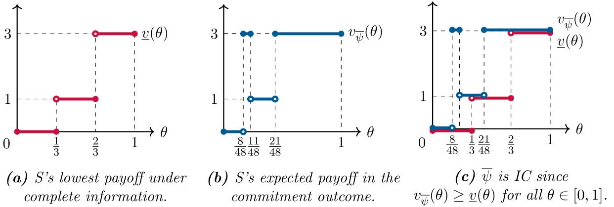
When $R$ chooses between two actions, $S$ always attains his commitment payoff in equilibrium.

Proposition 3. If $\Theta$ is rich and $|J| = 2$, then there exists a commitment outcome that is an equilibrium outcome.

Proof. By Proposition 2, there exists a deterministic commitment outcome $\bar{\psi}$. Using the same argument as that used in the proof of Proposition 1, we construct a deterministic commitment outcome $\tilde{\psi}$ that is IC. By Proposition 2, $\tilde{\psi}$ is an equilibrium outcome. $\square$

4.2. Finite state space

When the state space is finite, i.e., $\Theta = \{1, \dots, N\}$, a deterministic commitment outcome may not exist. For instance, in Example 1, the unique commitment outcome is not deterministic. As a result, $S$ may not be able to achieve the commitment payoff in equilibrium.

However, here we show that when the state space is sufficiently rich (in the sense that $\mu_0(\theta)$ is sufficiently small for each $\theta \in \Theta$), then $S$ 's equilibrium payoff approaches his commitment payoff. For a concise argument, we adopt the assumptions of Alonso and Câmara (2016): $R$ has a binary action and

where $\delta(\theta) = u(2, \theta) - u(1, \theta)$ for all $\theta \in \Theta$.

Proof. If $A_2 = \Theta$, then let $\alpha(2 | \theta) = 1$ for all $\theta \in \Theta$ so that $V_\alpha = V^*$. Thus, we assume for the remainder of the proof that $A_2$ is a proper subset of $\Theta$. Since (RU) holds, we can use Proposition 2 in Alonso and Câmara (2016) to find a cutoff state $\theta^* \in \Theta$ such that $\delta(\theta^*) < 0$ and, for every commitment outcome $\psi$, we have $\psi(2 | \theta) = 1$ ($\psi(1 | \theta) = 1$) for all $\theta \in \Theta$ such that $\delta(\theta) > \delta(\theta^*)$ ($\delta(\theta) < \delta(\theta^*)$). Now consider a deterministic outcome $\alpha$ with partition $\{W_1, W_2\}$ such that $W_2 = \{\theta \in \Theta | \psi(2 | \theta) = 1\}$ and $W_1 = \Theta \setminus W_2$. It is easy to see that $\alpha$ is IC and obedient, and therefore it is an equilibrium outcome by Theorem 1. If $\psi(2 | \theta^*) = 1$, the difference in $S$ 's ex-ante payoffs is zero; otherwise, we have $V^* - V_\alpha = \psi(2 | \theta^*)\mu_0(\theta^*) < \mu_0(\theta^*) < \gamma := \varepsilon$. $\square$

Thus, when $R$ chooses between two actions, $S$ can attain a payoff arbitrarily close to his commitment payoff in equilibrium as long as the prior probability of each state is sufficiently small.

5. A model with a stochastic message mapping

Definition 4. A triple $(\widehat{\sigma}, \widehat{\tau}, \widehat{q})$, where $\widehat{\sigma} : \Theta \times [0, 1] \rightarrow \Delta_0 \widehat{M}$ is S's strategy, $\widehat{\tau} : \widehat{M} \rightarrow \Delta J$ is R's strategy, and $\widehat{q} : \widehat{M} \rightarrow \Delta \Theta$ is R's belief system, is an equilibrium of the SMM game if

1. for all $\theta \in \Theta$ and $x \in [0, 1]$, $\widehat{\sigma}(\cdot | \theta, x)$ is supported on $\arg \max_{\{m \in \widehat{M} | x \in m\}} \sum_{j \in J} v(j) \widehat{\tau}(j | m)$;
2. for all $m \in \widehat{M}$, $\widehat{\tau}(\cdot | m)$ is supported on $\arg \max_{j \in J} \int_{\Theta} u(j, \theta) d\widehat{q}(\theta | m)$;
3. $\widehat{q}$ is obtained from $\mu_0$, given $\widehat{\sigma}$, using Bayes' rule;
4. for all $m \in \widehat{M}$, $\widehat{q}(\cdot | m) \in \Delta\{\theta \in \Theta | X^\theta \cap m \neq \emptyset\}$.

Since $x$ is payoff-irrelevant, an outcome $\alpha$ of the SMM game is an element of $\Psi$. An outcome $\alpha$ is an equilibrium outcome of the SMM game if an equilibrium $(\widehat{\sigma}, \widehat{\tau}, \widehat{q})$ exists that induces it, i.e., $\alpha(j | \theta) = \int_{X^\theta} \sum_{m \in \text{supp } \widehat{\sigma}(\cdot | \theta, x)} \widehat{\sigma}(m | \theta, x) \widehat{\tau}(j | m) dx / \mu_0(\theta)$.

We derive a sharp characterization of equilibrium outcomes in the SMM game.

Theorem 3. Let $\Theta$ be finite. Then $\alpha \in \Psi$ is an equilibrium outcome of the SMM game $\iff \alpha$ is IC and obedient.

Proof. $(\implies)$ is proved exactly the same way as Theorem 1 Part 1. An equilibrium outcome must be IC or else S has a profitable deviation to fully revealing $x$ (which also reveals $\theta \in \Theta$ since $x \in X^\theta$). An equilibrium outcome must be obedient by Bayes' rule.

$(\impliedby)$ Consider an IC and obedient outcome $\alpha$. For every $\theta \in \Theta$, let $J^\theta := \text{supp } \alpha(\cdot | \theta)$ be the set of actions that R takes with a positive probability when the realized state is $\theta$. Next, partition $X^\theta$ into a set of intervals $\{X_j^\theta\}_{j \in J^\theta}$ such that $\lambda(X_j^\theta) / \lambda(X^\theta) = \alpha(j | \theta)$. Also, for each action $j \in J$, let $W_j := \bigcup_{\theta \in \Theta} X_j^\theta$; by construction, $\{W_j\}_{j \in J}$ is a partition of $[0, 1]$.

Now let S's strategy be $\widehat{\sigma}(m | \theta, x) = \mathbb{1}(m = W_j \text{ and } x \in W_j)$. Then R's posterior after an on-path message $W_j$ is $\widehat{q}(\theta | W_j) = \lambda(X_j^\theta) / \lambda(W_j)$. Furthermore, since $\alpha$ is obedient, for every action $j \in J$ such that $\lambda(W_j) > 0$, we have

meaning that R prefers to take action $j$ after message $W_j$, so we let $\widehat{\tau}(j | W_j) = 1$. Off the path, let R be "skeptical" and assume that any unexpected message comes from the state in which S benefits from such deviation the most. Formally, for all $m \notin \{W_j\}_{j \in J}$, let $\widehat{q}(\cdot | m) \in \Delta A_j$, where $j \in J$ is the lowest action such that $m \cap X^\theta \neq \emptyset$ and $\theta \in A_j$. Then playing action $j$ is a best response to message $m$, so we let $\widehat{\tau}(j | m) = 1$. Since $\alpha$ is IC, S does not have profitable deviations by the same argument as in the proof of Theorem 1. Deviations to on-path messages are not available because $\{W_j\}_{j \in J}$ is a partition, and deviations to off-path messages are not profitable since the payoff from any deviation in state $\theta$ is at most $\underline{v}(\theta)$, which is below $v_\alpha(\theta)$ by the (IC $_\theta$) constraint. Hence, $(\widehat{\sigma}, \widehat{\tau}, \widehat{q})$ is an equilibrium of the SMM game. $\square$

In contrast to Theorem 1, IC and obedience are necessary and sufficient for an outcome to be an equilibrium outcome of the SMM game. Two properties of the SMM game ensure that every IC and obedient outcome is an equilibrium outcome. First, S's message space depends on $x$, which means S may receive different equilibrium payoffs in some state $\theta$ (but for different realizations of $x$). Second, the message space is "rich," meaning that for every vector $p = (p_1, \dots, p_N) \in [0, 1]^N$, there exists a message $m$ that is available in state $\theta \in \Theta$ with probability $p_\theta$. This richness allows us to "purify" any nondeterministic outcome: the equilibria that we construct to implement an IC and obedient outcome is in pure strategies of both S and R.

Using the sharp equilibrium characterization of the SMM game, we derive the following results.

Corollary 1. Let $\Theta$ be finite. Then a commitment outcome is an equilibrium outcome of the SMM game if and only if it is IC.

Corollary 2. If $\Theta$ is finite and $|J| = 2$, then every commitment outcome is an equilibrium outcome of the SMM game.

Corollary 1 is a direct consequence of Theorem 3. Corollary 2 follows from Theorem 3 and the fact that every commitment outcome is IC when R has two actions (see Alonso and Câmara, 2016 and our discussion after Proposition 1).

The set of equilibrium outcomes in the SMM game coincides with the set of IO outcomes found in KS if S's value function is quasiconvex in R's belief (KS Proposition 3), or when R chooses between two actions (KS Proposition 4). Generally, the set of IO outcomes is a subset of the set of equilibrium outcomes in KS, because IO imposes a stronger restriction on off-path beliefs than our equilibrium concept.

6. Conclusion

This paper examined a persuasion game with verifiable information in which a sender with transparent motives chooses which verifiable messages to send to a receiver in order to convince her to take a particular action from a finite set. We showed that every equilibrium outcome must be incentive-compatible for the sender and obedient for the receiver. If an outcome is deterministic, then these conditions are both necessary and sufficient for it to be an equilibrium outcome. We also identified sufficient conditions under which the ex-ante commitment assumption in Bayesian persuasion can be replaced by communication with verifiable information. We showed that if the state space is rich, then a deterministic commitment outcome always exists; this commitment outcome is an equilibrium outcome if and only if the sender receives at least his complete information payoff in every state. If the receiver chooses between two actions, this condition is automatically satisfied. We hope these results prove useful in applied settings.

Data availability

No data was used for the research described in the article.

CRediT authorship contribution statement

Maria Titova: Writing – review & editing, Writing – original draft; Kun Zhang: Writing – review & editing, Writing – original draft.

Declaration of competing interest

None

References

• Ali, S.N., Kleiner, A., Zhang, K., 2024. From design to disclosure. Working paper.
• Alonso, R., Câmara, O., 2016. Persuading voters. 106 (11), 3590–3605. https://doi.org/10.1257/aer.20140737
• Bardhi, A., Guo, Y., 2018. Modes of persuasion toward unanimous consent. 13 (3), 1111–1149. https://doi.org/10.3982/TE2834
• Ben-Porath, E., Dekel, E., Lipman, B.L., 2019. Mechanisms with evidence: commitment and robustness. 87 (2), 529–566. https://doi.org/10.3982/ECTA14991
• Boleslasky, R., Cotton, C., 2015. Grading standards and education quality. 7 (2), 248–279. https://doi.org/10.1257/mic.20130080
• Bull, J., Watson, J., 2007. Hard evidence and mechanism design. 58 (1), 75–93. https://doi.org/10.1016/j.geb.2006.03.003
• Chakraborty, A., Harbaugh, R., 2010. Persuasion by cheap talk 100 (5), 2361–2382. https://doi.org/10.1257/aer.100.5.2361
• Dranove, D., Jin, G.Z., 2010. Quality disclosure and certification: theory and practice. J. Econ. Lit. 48 (4), 935–963.
• Dvoretzky, A., Wald, A., Wolfowitz, J., 1951. Elimination of randomization in certain statistical decision procedures and zero-sum two-person games. Ann. Math. Stat. 22 (1), 1–21. https://doi.org/10.1214/aoms/1177729689
• Dye, R.A., 1985. Disclosure of nonproprietary information. J. Accounting Res., 23 (1), 123–145.
• Gehlbach, S., Sonin, K., 2014. Government control of the media. 118, 163–171. https://doi.org/10.1016/j.jpubeco.2014.06.004
• Gentzkow, M., Kamenica, E., 2016. A Rothschild-Stiglitz approach to Bayesian persuasion. 106 (5), 597–601. https://doi.org/10.1257/aer.p20161049
• Gieczewski, G., Titova, M., 2024. Coalition-proof disclosure. Working paper.
• Glazer, J., Rubinstein, A., 2004. On optimal rules of persuasion. Econometrica 72 (6), 1715–1736. https://doi.org/10.1111/j.1468-0262.2004.00551.x
• Glazer, J., Rubinstein, A., 2006. A study in the pragmatics of persuasion: a game theoretical approach. Theor. Econ. 1, 395–410. http://econtheory.org/j.ctt46mwfz.9
• Grossman, S.J., The informational role of warranties and private disclosure about product quality. 1981. 24 (3), 461–483. https://doi.org/10.1086/466995
• Grossman, S.J., Hart, O.D., 1980. Disclosure laws and takeover bids. J. Finance 35 (2), 323–334.
• Hart, S., Kremer, I., Perry, M., 2017. Evidence games: truth and commitment. Am. Econ. Rev. 107 (3), 690–713. https://doi.org/10.1257/aer.20150913
• Kamenica, E., Gentzkow, M., 2011. Bayesian persuasion. 101 (6), 2590–2615. https://doi.org/10.1257/aer.101.6.2590
• Kamenica, E., Lin, X., 2024. Commitment and randomization in communication. arXiv preprint arXiv:2410.17503.
• Koessler, F., Renault, R., 2012. When does a firm disclose product information? Rand J. Econ. 43 (4), 630–649. https://www.jstor.org/stable/41723348
• Koessler, F., Skreta, V., 2023. Informed information design. https://doi.org/10.1086/724843
• Kolotilin, A., 2015. Experimental design to persuade. 90, 215–226. https://doi.org/10.1016/j.geb.2015.02.006
• Lipnowski, E., 2020. Equivalence of cheap talk and Bayesian persuasion in a finite continuous model. Working paper.
• Lipnowski, E., Ravid, D., 2020. Cheap talk with transparent motives. 88 (4), 1631–1660. https://doi.org/10.3982/ECTA15674
• Milgrom, P.R., 1981. Good news and bad news: representation theorems and applications. 12 (2), 380. https://doi.org/10.2307/3003562
• Milgrom, P.R., 2008. What the seller won't tell you: persuasion and disclosure in markets. 22 (2), 115–131. https://doi.org/10.1257/jep.22.2.115
• Milgrom, P.R., Roberts, J., et al., 1986. Relying on the information of interested parties. 17 (1), 18. https://doi.org/10.2307/2555625
• Ostrovsky, M., Schwarz, M., 2010. Information disclosure and unraveling in matching markets. 2 (2), 34–63. https://doi.org/10.1257/mic.2.2.34
• Perez-Richet, E., 2014. Interim Bayesian persuasion: first steps. Am. Econ. Rev. 104 (5), 469–474.
• Sher, I., 2011. Credibility and determinism in a game of persuasion. Games Econ. Behav. 71 (2), 409–419. https://doi.org/10.1016/j.geb.2010.05.008
• Terstiege, S., Wasser, C., 2023. Experiments versus distributions of posteriors. Math. Soc. Sci. 125, 58–60.
• Zapechelnuk, A., 2023. On the equivalence of information design by uninformed and informed principals. Econ. Theory 76 (4), 1051–1067. https://doi.org/10.1007/s00199-023-01495-z
• Zhang, K., 2022. Withholding verifiable information. Working paper.