Withholding Verifiable Information
Revision requested by Theoretical Economics
We study a class of finite-action disclosure games in which the sender's preferences are state-independent and the receiver's optimal action depends only on the expected state. While receiver-preferred equilibria in these games involve full revelation, other equilibria are less well understood. We show that any equilibrium payoff can be obtained with a disclosure strategy corresponding to a partition with a laminar structure that allows pooling of nonadjacent states. In a sender-preferred equilibrium, such a structure balances inducing more sender-favorable actions with deterring deviations. Leveraging this insight, we identify conditions under which the sender does not benefit from commitment power. We then apply these results to study selling with quality disclosure and influencing voters.
@unpublished{WVI,
  author = {Denis Shishkin and Maria Titova and Kun Zhang},
  title = {Withholding Verifiable Information},
  year = {2026},
  url = {https://arxiv.org/abs/2206.09918},
}
Abstract
We study a class of finite-action disclosure games in which the sender's preferences are state-independent and the receiver's optimal action depends only on the expected state. While receiver-preferred equilibria in these games involve full revelation, other equilibria are less well understood. We show that any equilibrium payoff can be obtained with a disclosure strategy corresponding to a partition with a laminar structure that allows pooling of nonadjacent states. In a sender-preferred equilibrium, such a structure balances inducing more sender-favorable actions with deterring deviations. Leveraging this insight, we identify conditions under which the sender does not benefit from commitment power. We then apply these results to study selling with quality disclosure and influencing voters.
1 Introduction
A canonical prediction in disclosure games is unraveling (e.g., Grossman, 1981; Milgrom, 1981). Specifically, if a sender can credibly prove that a state is highly favorable, he reveals it to induce a higher action from a receiver. Once the most favorable states have been disclosed, slightly less favorable states must also be revealed to avoid being mistaken for worse ones, and this reasoning continues recursively until all states are revealed. This full-revelation result hinges on a crucial assumption: the receiver’s action space is sufficiently flexible, meaning that she can adjust her action continuously so that any marginal improvement in her belief leads to a strictly higher action.
However, this flexibility assumption often fails in settings where the receiver chooses among finitely many actions—for example, when a consumer decides between a few products or product versions or a policymaker chooses among a few policy alternatives. In such cases, the receiver cannot finely adjust her action in response to small changes in her belief. Previous studies (e.g., Giovannoni and Seidmann, 2007; Titova and Zhang, 2025) have shown that this discreteness may prevent full unraveling and allow the sender to withhold some information—that is, create a scope for pooling. Yet little is known about precisely which states are pooled in equilibrium or about the limits of what can be achieved through verifiable disclosure.
In this paper, we study a disclosure game in which the receiver’s preferred action is increasing in the expected state. The only essential difference from Milgrom (1981) is that our receiver’s action space is finite. We characterize the equilibrium payoff set, study the sender-preferred equilibrium payoff, and identify sufficient conditions under which the commitment payoff is achieved with verifiable disclosure. We illustrate our results with a motivating example.
Example. Consider a seller (he) promoting a product to a buyer (she) who chooses whether to buy nothing (action 1), buy the product (action 2), or buy the product bundled with an add-on (action 3). The players have a common prior that the product quality—which can be interpreted as either the sender’s type or the state of the world—is uniformly distributed on . The buyer’s payoff depends on the posterior expectation of product quality and is such that she optimally buys the bundle if , only the standalone product if , and nothing otherwise. The seller’s profit is 0 if he sells nothing, 1 if he sells the product with the add-on, and if he sells the product only. To persuade the buyer, the seller can disclose a piece of hard evidence about product quality after privately observing it. In particular, he can send a message corresponding to any nonempty closed subset of containing the true quality . We focus on partitional disclosure strategies associated with some (ordered) partition of such that when the product quality is , the seller sends a message , which is interpreted as a recommendation for the buyer to take action . To determine whether a partition can arise in an equilibrium, one needs to ensure that no player can profitably deviate. First, the partition must satisfy obedience in the sense that the buyer is willing to follow the recommendation. Second, it must satisfy revelation proofness in the sense that the seller is never willing to deviate by revealing the true quality. One can show that these properties are not only necessary but also sufficient for a partitional strategy to be an equilibrium strategy.
First, note that the seller's equilibrium payoff is bounded from above by his commitment payoff in this environment—that is, his maximal expected payoff in the case in which he can commit to disclosing information about using any experiment. The commitment problem can be seen as a relaxation of the problem of maximizing the seller's payoff across equilibria because the former does not require the disclosure strategy to be revelation-proof. Therefore, if the commitment payoff is attainable in some equilibrium, this equilibrium must be a seller-preferred equilibrium of the game.
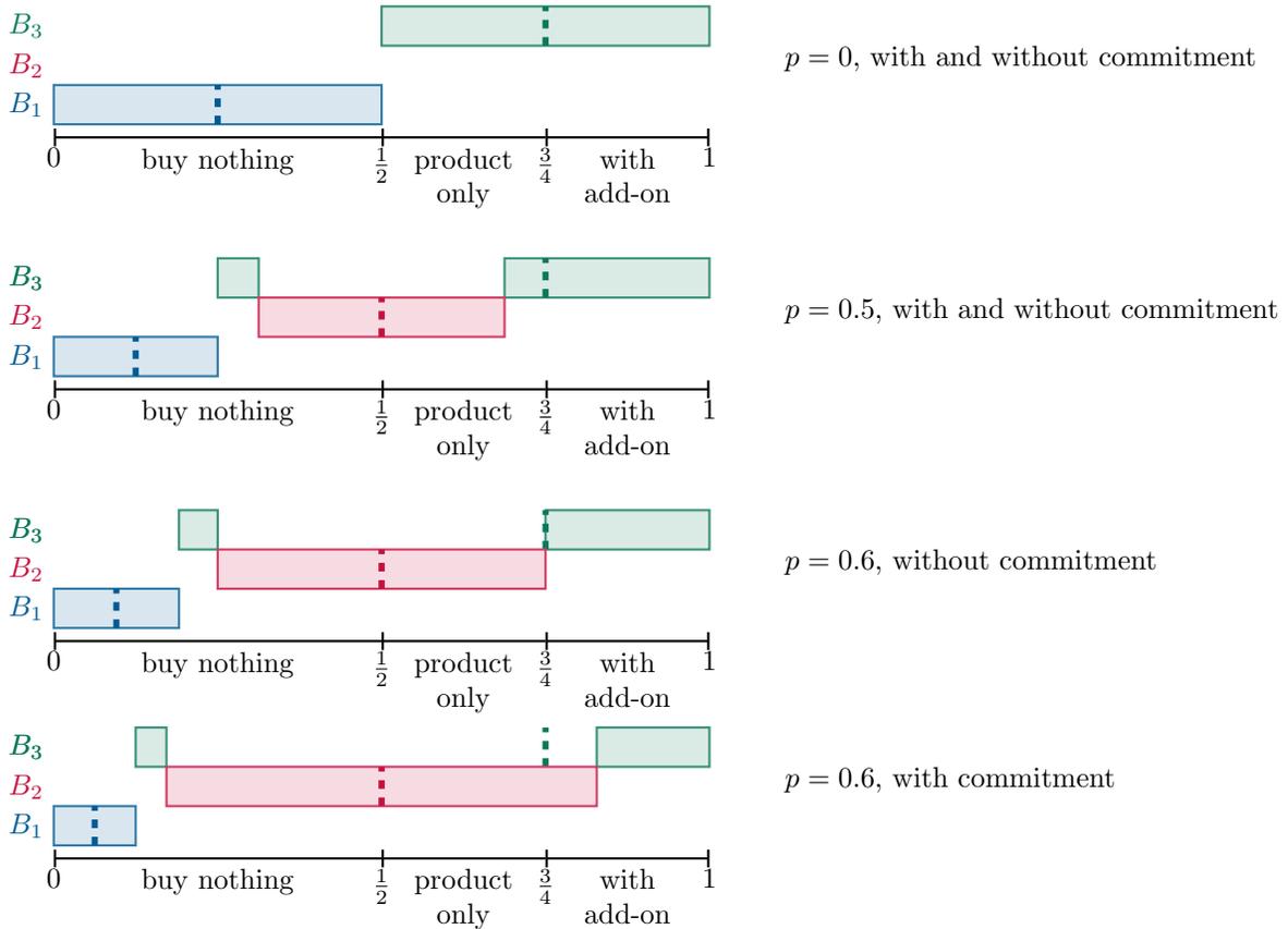
Suppose first that . Given the observation above, we start by identifying the commitment solution. Because , the action space is effectively binary and the seller is maximizing the probability of selling the bundle. Every commitment-optimal experiment corresponds to a partition given by , , so that the buyer is indifferent between buying and not buying the bundle following message . It is easy to check that this partition is revelation-proof, as no seller type in can induce any action higher than 1 by deviating. We have thus found a seller-preferred equilibrium that attains the commitment payoff.
Suppose next that . In this case, there are three nontrivial actions available to the buyer, and the seller faces a trade-off between the likelihood of selling the standalone product and the likelihood of selling the bundle. It turns out that the unique commitment-optimal partition is given by , , (see Figure 1). Note two important properties of this partition. First, while this partition must satisfy obedience, it does so only barely, in the sense that the means of and are the lowest posterior means compatible with obedience. Namely, their means are exactly the cutoffs and for actions 2 and 3, respectively. Intuitively, if the obedience constraint were slack, the seller would be able to perturb the partition and shift the probability toward higher actions. Second, in contrast to the case of , the optimal partition here is not monotone in the sense that some elements are not intervals. Instead, it is associated with a class of bi-pooling distributions of posterior means, which are known to be optimal in a general class of linear persuasion problems (Kleiner, Moldovanu, and Strack, 2021; Arieli, Babichenko, Smorodinsky, and Yamashita, 2023). Such bi-pooling partitions generalize monotone partitions by allowing pooling of nonadjacent types as follows. Each partitional element is an interval or consists of two intervals and “nests” a unique other interval in the sense that . Intuitively, such bi-pooling partitions arise as commitment optima because among barely obedient partitions they always allow for optimally resolving the trade-off between the likelihoods of difference actions. To determine whether the commitment payoff is attainable in equilibrium, we need to verify that this partition is revelation-proof. It is sufficient to check that no type in can deviate by revealing their type and convincing the buyer to buy the bundle. Indeed, since the highest type in is below the threshold of selling a bundle, this partition is a seller-preferred equilibrium partition.
Suppose next that . The unique commitment-optimal partition can be shown to be given by a bi-pooling partition , , . Compared to the previous case, here the profit from selling the standalone product expands and the set of types selling the standalone product shrinks. In particular, there are now some types in that are above the bundle threshold of and for whom revealing their type would be a profitable deviation. Therefore, the above partition is not revelation-proof and the maximal equilibrium seller profit in the disclosure game is strictly below the commitment benchmark. In this case, the seller-optimal equilibrium turns out to be associated with another bi-pooling partition given by , , . To see why the seller cannot do better in equilibrium, note that this partition has two constraints. First, it is barely obedient for the same reason as the commitment optima described above. Second, in contrast to the commitment solution, the upper bound of coincides with the threshold , indicating that the seller revelation-proofness constraint is binding.
Our model generalizes this example to any absolutely continuous prior distribution of the state, an ordered finite action space, and monotone preferences of the players.1
Our first main result, Theorem 1, characterizes the sender's equilibrium payoff set by showing that every equilibrium payoff can be obtained in a laminar partitional equilibrium, that is, one associated with a laminar partition. The laminar property of a partition, introduced in Candogan and Strack (2023), generalizes the aforementioned bi-pooling property as follows. In a bi-pooling partition, each element's convex hull may nest at most one other lower-indexed element, while in a laminar partition, it may nest any number of lower-indexed elements. The key step in the characterization is showing that laminar partitions are the most revelation-proof among all obedient partitions in the sense that any equilibrium partition can be transformed into a laminar equilibrium partition with the same sender payoff.
Our next result, Theorem 2, characterizes sender-preferred laminar equilibrium partitions and, more generally, provides a sharp equilibrium test for barely obedient laminar partitions. First, sender-preferred laminar equilibrium partitions are barely obedient in the sense that they leave no slack in the receiver’s obedience constraints. Theorem 2 also bounds their complexity by showing that action is recommended on at most intervals of states. Finally, for barely obedient laminar partitions, revelation proofness is simplified into a local condition: it suffices to check only a small subset of the non-lowest on-path actions and only at the highest state recommend each such action. In all other cases, revelation proofness is automatic.
Our remaining set of results discusses the attainability of the commitment payoff in the disclosure game. It is well known that generically every commitment problem admits a unique bi-pooling solution. We establish in Theorem 3 that, among all partitions yielding this solution, there is a unique barely obedient bi-pooling one. Moreover, this partition is most resistant to violations of revelation proofness; consequently, the revelation proofness of this partition determines whether the commitment payoff can be achieved in a disclosure game (Proposition 1). With binary actions, Titova and Zhang (2025) show that every bi-pooling commitment solution is implementable. Our Proposition 2 shows that for three or more actions, every bi-pooling commitment solution is implementable if the sender’s utility is sufficiently convex in the cutoffs for the receiver’s actions. In the above example with three actions, the sender’s utility is sufficiently convex when is sufficiently low.
Our results suggest that full revelation may not be the only relevant outcome, even in settings where the sender can prove any true fact. In particular, when the receiver has only finitely many actions, the emergence of a rich set of simple equilibria can help explain the variety of disclosure policies observed in practice. Even within the class of laminar partitional equilibria, the same environment can sustain a fully revealing equilibrium, a sender-preferred equilibrium with substantially more withholding of information, and every payoff in between. Our analysis of sender-preferred equilibria also informs the case of mandatory disclosure: in some environments, voluntary disclosure may lead to pooling of a large fraction of low states with high states and therefore a much lower receiver’s payoff.
We apply these insights to study selling with quality disclosure and influencing voters. In the former setting, Milgrom (1981) shows that when the buyer can purchase any fraction of the product, unraveling takes place and every equilibrium features full revelation. We show that if the buyer is restricted to purchasing integer units, the seller may be able to achieve the commitment payoff by withholding information. In the second application, we consider an expert who discloses verifiable information to a voter who chooses from three alternatives: the amended bill, the unamended bill, and the status quo. We demonstrate that the expert can be hurt even if, all else equal, the voter becomes more inclined toward the expert’s most preferred alternative.
Related literature. This paper belongs to a growing body of literature that characterizes the equilibrium payoff set in disclosure games.2 The most closely related paper is Titova and Zhang (2025), which studies a more general disclosure game with a finite number of receiver actions. We specialize their model by assuming the state space is the unit interval and the receiver has monotonic preferences that depend only on the expected state. These assumptions allow us to characterize sender-preferred equilibria, identify the limits of verifiable communication, and establish sufficient conditions on model primitives under which the sender achieves the commitment payoff. While we focus on environments in which the receiver’s action set is more limited than it is in Grossman (1981) and Milgrom (1981)—our receiver chooses from a finite set of actions—Ali, Kleiner, and Zhang (2024) study settings with greater flexibility, where full revelation prompts an action that makes the sender no better off than inducing any other beliefs. Consequently, revelation proofness is not a concern. They provide conditions under which the set of equilibrium payoff profiles is virtually the same as the set of achievable payoff profiles under commitment. Gieczewski and Titova (2025) consider disclosure games with a general message mapping, propose an equilibrium selection criterion related to neologism proofness, and characterize the sender’s ex-ante payoffs under this criterion when the sender has access to sufficiently rich stochastic evidence.3
Beyond expanding the work on disclosure games, our work contributes to the growing body of literature on the possibility of attaining the commitment payoff without full commitment in other communication environments, as in the cases of cheap talk (Lipnowski and Ravid, 2020; Lipnowski, 2020), repeated cheap talk (Best and Quigley, 2024; Kuvalekar, Lipnowski, and Ramos, 2022; Mathevet, Pearce, and Stacchetti, 2022; Pei, 2023), informed information design (Perez-Richet, 2014; Koessler and Skreta, 2023; Zapechelnyuk, 2023),4 the ability to covertly revise a message generated by an experi-ment (Min, 2021; Lipnowski, Ravid, and Shishkin, 2022), the ability to covertly revise an experiment without affecting the marginal distribution over messages (Lin and Liu, 2024), costly misreporting (Guo and Shmaya, 2021; Nguyen and Tan, 2021), disclosure following private experimentation (Arieli and Stewart, 2025; Dai, Fudenberg, and Pei, 2026), and Bayesian persuasion under sender-worst equilibrium selection (Lipnowski, Ravid, and Shishkin, 2025). In contrast to these studies, we study a one-shot communication game with verifiable information without any commitment.
In the literature, pooling of nonadjacent states has been obtained in settings with either sender commitment (e.g., Kleiner et al., 2021; Arieli et al., 2023), the receiver’s private information (e.g., Feltovich, Harbaugh, and To, 2002; Harbaugh and To, 2020)5, or both (e.g., Guo and Shmaya, 2019; Candogan and Strack, 2023). While our setting has neither sender commitment nor receiver private information, equilibria in our game feature a similar structure. The most closely related paper to ours is Candogan and Strack (2023), which studies linear persuasion with one or more privately informed receivers. In that paper, laminar partitions arise as solutions to standard linear maximization problems with a mean-preserving contraction constraint, in which the receivers’ incentive constraints are written as additional moment conditions. Despite the fact that our revelation-proofness constraint cannot be written as a moment condition, the laminar property likewise plays a key role in our disclosure game because, as we show, laminar partitions turn out to be the most revelation-proof.
2 The Model
We consider the following disclosure game between the sender (he) and the receiver (she).6 The state space is , and the common prior belief is induced by a CDF that admits a strictly positive density . First, the sender learns the state. Then the sender communicates with the receiver using verifiable messages. Specifically, the sender’s message space in state is , where is the collection of all nonempty closed subsets of . Finally, the receiver observes the message, forms a posterior belief, and takes an action.
The receiver’s action space is , where . The receiver’s optimal evidence. action depends only on her posterior mean, denoted by . We assume that the receiver's preferences are monotone in the sense that action is optimal if and only if for some cutoffs .7 We also assume that the sender's state-independent payoff from the receiver taking action is strictly increasing in .8 Without loss, we normalize . Finally, let
denote the sender's value function, which maps the receiver's posterior mean to the highest attainable sender payoff. By construction, is upper semicontinuous.
We focus on perfect Bayesian equilibria of the disclosure game. An assessment is a triple , where is the sender's strategy, is the receiver's strategy, and is the receiver's belief system.9 An assessment is a (perfect Bayesian) equilibrium if
- for every , is supported on ;
- for every , implies ;
- is obtained from given using Bayes' rule;
- for every , .
In words, the first condition requires that the sender choose verifiable messages that maximize his expected payoff. The second condition requires that the receiver chooses an action that is optimal given her posterior mean. The third condition requires that the receiver uses Bayes' rule to calculate posterior beliefs from the prior and the sender's strategy. The final condition requires that the receiver's belief system is consistent with disclosure: she deems impossible any state in which the observed (on- or off-path) message is unavailable.
3 Equilibrium Analysis
We begin the analysis by introducing the notion of a partition of the state space and its key properties. A sequence of closed subsets of is an (ordered) partition if and for all . Note that we index partitions using the action set for notational convenience; we also allow partitional elements to have nonempty but null intersections.
We say that an assessment and a partition are associated if for each ,
- (a) ;
- (b) ;
- (c) .
In an assessment associated with a partition , the sender's strategy is to reveal which element of the partition the state belongs to by sending message when .10 Such a message can be interpreted as a recommendation for the receiver to choose action . Then the receiver's strategy is to always follow the recommendation. Finally, the receiver's posterior beliefs on the path are computed using Bayes' rule. Note that a partition uniquely defines the players' on-path behavior: if a partition is associated with multiple assessments, all of those assessments differ only in the receiver's off-path beliefs and actions. If an assessment associated with a partition is an equilibrium, then we call a partitional equilibrium and an equilibrium partition. The following two properties are necessary and sufficient for to be an equilibrium partition.11
Definition 1. A partition is
- obedient if for each .
- revelation-proof if implies for each .
In words, obedience requires that the receiver indeed prefers to take action when she learns that , that is, after message . Revelation proofness ensures that fully revealing the state is not a profitable deviation for the sender. Indeed, in the disclosure game, the sender has the option to fully reveal the state by sending message with probability one, thus convincing the receiver to take the action that she would take knowing . Thus, if —in other words, the partition prescribes that the receiver takes action when the realized state is —then the receiver prefers to take at most action when fully informed.
Next we define a key structural property of partitions. Let and denote the closure and the convex hull operators, respectively.
Definition 2. A partition is laminar if for each ,
If an equilibrium is associated with a laminar partition , we call this equilibrium a laminar partitional equilibrium.
The intuitive interpretation of the laminar property is that each element either has no “gaps” and is therefore an interval or has “gaps” and these gaps belong to lower-indexed partitional elements only. This implies that for each pair and with , the convex hull either nests or has a null intersection with .12 When , we say that action nests action . We illustrate this intuition in Figure 2.
The following observation is a direct consequence of the definition of a laminar partition.
Observation 1. If is a laminar partition, then each is either an empty set or a union of at most intervals.
One prominent example of an obedient and revelation-proof laminar partition is , which we call the fully informative partition. Note that while is not fully revealing, it provides the minimal information necessary for the receiver to take her complete-information optimal action in each state.

Equilibrium Payoff Set
Next we turn to the characterization of the equilibrium payoff set. We say that an equilibrium is sender-preferred if it yields the highest ex-ante payoff for the sender across all equilibria. Analogously, we refer to the ex-ante payoff-minimizing equilibrium as sender-worst. Our first main result shows that every equilibrium ex-ante payoff of the sender is achievable in an equilibrium associated with an obedient and revelation-proof laminar partition.13
- Theorem 1.** (a) There exists a sender-worst equilibrium that is associated with the fully informative partition and yields .
- (b) There exists a sender-preferred equilibrium that is associated with an obedient and revelation-proof laminar partition and yields .
- (c) For any , there exists an equilibrium associated with an obedient and revelation-proof laminar partition.
We provide the intuition for Theorem 1 below. Part (a) is straightforward: as in most disclosure games, there exists an equilibrium in which the receiver acts as if she is fully informed. In our setting, that equilibrium is associated with the fully informative partition . The sender's ex-ante payoff cannot fall below , or else the sender will have a profitable deviation toward fully revealing some state.
Part (b) follows from two key observations. First, note that it is without loss to focus on partitional equilibria. This is because in a sender-preferred equilibrium, the receiver breaks ties in favor of the sender. Hence, a single action is taken with probability one in each state.
Second, we show that for any equilibrium partition there exists an equilibrium laminar partition that induces the same posterior mean distribution (PMD) and hence yields the same ex-ante payoff to the sender. We first observe that any partition induces a PMD with support on at most points (posterior means); using the techniques from Candogan and Strack (2023), we show that any such PMD can be induced by a laminar partition. We further show that if a PMD is induced by an obedient and revelation-proof partition, then the laminar partition that induces the same PMD is guaranteed to be obedient and revelation-proof. In this sense, laminar partitions are the most revelation-proof partitions.
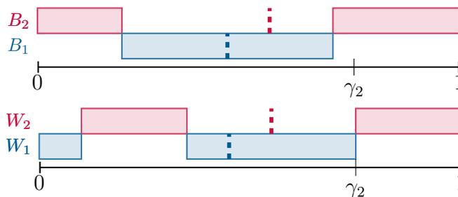
We illustrate the intuition behind laminar partitions as the most revelation-proof ones in Figure 3, which presents the simplest case, where . Consider two partitions, (laminar) and (non-laminar), that induce the same PMD and whose corresponding elements have the same prior mass; that is, and for all . Since is laminar, its lowest-indexed element is an interval. If is not an interval, the only way to match 's prior mass and expectation is to have . Consequently, if is revelation-proof (which, in the case of two actions, reduces to ), so is .
Combining the two aforementioned observations, to solve for the sender-preferred equilibrium payoff, one can maximize the sender's expected payoff across all obedient and revelation-proof laminar partitions as follows:
subject to: is an obedient and revelation-proof laminar partition.
We show that problem (2) admits a solution,14 which implies that a sender-preferred equilibrium exists. To show that , we construct an obedient and revelation-proof (and hence equilibrium) laminar partition that yields a strictly higher payoff than . For example, take the fully revealing partition and “move” the interval from the first element of the partition to the -th one. If is sufficiently small, the resulting partition will remain obedient, revelation-proof, and laminar, but the sender’s ex-ante utility in the associated equilibrium will be strictly higher than . Therefore, the sender’s ex-ante payoff in his most preferred equilibrium will also exceed .
To prove Part (c), we show that for any payoff between and there exists a laminar equilibrium partition that blends the sender-worst (fully informative and laminar) partition and the sender-preferred laminar equilibrium partition , and this blend yields the payoff.
Sender-Preferred Equilibrium
Next we characterize the sender-preferred laminar partitional equilibrium. We say that action is skipped in partition if is a null set and unskipped otherwise. We refer to partition as barely obedient if for all but the lowest unskipped .
Theorem 2. Every sender-preferred laminar equilibrium partition is barely obedient, and is the union of at most closed intervals for all . Furthermore, a barely obedient laminar partition is an equilibrium partition if and only if for any unskipped action such that action either nests or is skipped.
The first part of Theorem 2 characterizes problem (2)’s solution—that is, an obedient and revelation-proof laminar partition that maximizes the sender’s ex-ante payoff. First, must be barely obedient; otherwise, one could pool additional low states with high states without violating obedience or revelation proofness, thereby obtaining an equilibrium with a strictly higher ex-ante sender payoff. Specifically, if is the lowest unskipped action, one can reassign a subset of of strictly positive measure to for some . To show that each partitional element is the union of at most closed intervals, we first note that for some for the lowest unskipped action . That is, the lowest unskipped action is an interval that is not in the convex hull of any other partitional elements. Then each partitional element with index must be a union of at most intervals by the definition of a laminar partition.
Next, note that revelation proofness is equivalent to for each action . The second part of Theorem 2 shows that for a barely obedient laminar partition, this constraint is only binding for an action in two specific scenarios, illustrated in Figure 4: either the next-highest action is skipped or the action's corresponding partitional element is nested within the convex hull of the partitional element for the next-highest action. In all other instances, revelation proofness is automatically satisfied. This finding further emphasizes that the laminar structure makes revelation proofness easier to fulfill.

As in Candogan and Strack (2023), the laminar structure emerges in a sender-preferred equilibrium of our game due to incentive constraints. In Candogan and Strack (2023), where the receiver is privately informed, the laminar structure prevents the receiver from misreporting her private information. In our setting, however, it optimally balances the trade-off between deterring the sender's deviations and inducing the most desirable action distribution.
As discussed after Theorem 1, laminar partitions are the most revelation-proof among all obedient partitions. However, interval partitions—a special case of laminar partitions—often fail to be sender-preferred equilibrium partitions. This underscores the importance of pooling nonadjacent states in inducing the most desirable distribution over actions subject to obedience and revelation proofness. To illustrate, recall our introductory example with . The interval partition that generates the highest sender's ex-ante payoff is given by , , . Since , we can pool the states from the top of with until the partition becomes barely obedient. This process yields a sender-preferred equilibrium partition, , , .
4 When Is Commitment Payoff Achievable?
While the extent to which the sender benefits from verifiable communication depends on the specific parameters, an upper bound on the sender's payoff is given by his commitment payoff—that is, his payoff when he can commit to what messages to send in each state. In this section, we identify conditions under which the sender can attain his commitment payoff in an equilibrium of the disclosure game.
4.1 Commitment Benchmark
We start by introducing the commitment problem, or information-design problem, as a benchmark. In this problem, the sender can commit to any experiment that reveals information about the state. An experiment is a mapping , where is a sufficiently rich signal space. For each state , a signal realizes according to . Because the receiver's optimal action only depends on the expected state, it is without loss to restrict attention to the class of experiments in which and each is calibrated to equal the induced posterior mean: . Such a calibrated experiment induces the PMD with CDF .
It is well known that a PMD is induced by some experiment if and only if is a mean-preserving contraction of the prior CDF .15 Consequently, the commitment problem can be stated as a maximization of the expected value with respect to the PMD,
where is the set of all mean-preserving contractions of . We call any solution to problem (3) a commitment solution and call the value of problem (3) the commitment payoff. Clearly, the commitment payoff is an upper bound of the sender's equilibrium payoff in the disclosure game.
Finally, we say that a commitment solution is implementable with verifiable messages, or simply implementable for short, if there is an equilibrium in which the sender's strategy induces the receiver's PMD .
We say that an experiment is associated with a partition if it maps almost every into the degenerate distribution centered on . In other words, such an experiment discloses only which element of the partition the state belongs to. In this case, we also say that the induced PMD is associated with this partition.
Next we define a refinement of the laminar property, which is key for optimality under commitment.
Definition 3. A laminar partition is a bi-pooling partition if for every , either is an interval or there exists a unique and .

While laminar partitions allow any with to be nested within , bi-pooling partitions allow only for a single such to be nested within (see Figure 5).
The following result regarding bi-pooling partitions is a direct consequence of the results in Kleiner et al. (2021), Candogan (2022), and Arieli et al. (2023). Say that the communication environment is generic if no three elements of the collection of points are collinear.
Theorem 3. There exists a commitment solution associated with a unique barely obedient bi-pooling partition. Moreover, the commitment solution is unique in generic communication environments.
Theorem 3 indicates that, despite the simplicity of bi-pooling partitions, there always exists a commitment solution associated with a bi-pooling partition. Moreover, under mild conditions, the unique commitment solution is associated with a bi-pooling partition.
4.2 Characterizing Implementability
The following result characterizes the implementability of a commitment solution associated with a bi-pooling partition.
Proposition 1. Let be a commitment solution associated with a bi-pooling partition . Then is implementable if and only if is revelation-proof.
It follows directly from Theorem 3 and Proposition 1 that in a generic communication environment, the unique commitment solution is implementable if and only if the associated bi-pooling partition is revelation-proof.
The “if” part of Proposition 1 is a direct consequence of Theorem 2 in Titova and Zhang (2025), which states that for a partition associated with a commitment solution, implementability is equivalent to revelation proofness. Our primary contribution in Proposition 1 is to show that of all sender strategies that induce a commitment solution, the one associated with a bi-pooling partition has the best shot at being an equilibrium strategy. Roughly, this stems from the fact that bi-pooling partitions are a special case of laminar partitions, which exhibit a similar property.
Proposition 1 is useful in that it suggests a “guess and verify” approach to finding the sender-preferred equilibrium. First, one finds the commitment solution using standard information-design methods. Second, one identifies the associated bi-pooling partition. If this partition proves to be revelation-proof, then the sender-preferred equilibrium has been successfully identified.
The next result, which is a corollary of Proposition 1 and Theorem 2, goes one step further: it reveals the exact features of bi-pooling partitions that fail revelation proofness and hence prevent the commitment solutions from being implementable.
Corollary 1. Let be a commitment solution associated with a bi-pooling partition . Then is implementable if and only if is such that for any unskipped action such that action either nests or is skipped.
Compared to the definition of revelation proofness, the condition in Corollary 1 is easier to verify when determining whether a commitment solution is implementable. It also allows us to identify sufficient conditions under which commitment has no value in the subsequent Section 4.3.
To illustrate this result, recall our introductory example with , , , , , , and uniform . When , there is a unique commitment solution associated with a bi-pooling partition given by , , . Note that the condition in Corollary 1 only applies to action 1 and is satisfied because . In other words, the commitment-optimal partition is revelation-proof because the sender cannot induce an action higher than 1 by fully revealing the state when it is in .
When , there is a unique commitment solution associated with a bi-pooling partition given by , , . Note that the condition in Corollary 1 only applies to action 2 and is satisfied because .
Proposition 1 and Corollary 1 might suggest that implementing a commitment solution associated with a bi-pooling partition is relatively simple: one needs only to ensure that no action is recommended more often than revelation proofness allows. Indeed, Titova and Zhang (2025) showed that when a receiver is choosing between two actions, revelation proofness is automatically satisfied. When there are three or more actions, however, the restriction imposed by revelation proofness can be substantial. We illustrated this in our introductory example with . In this case, the commitment-optimal bi-pooling partition is given by , , . Note that in this case the condition in Corollary 1 is violated for action 2, which is nested by action 3, but .
When there are two actions, the sender’s sole objective is to maximize the probability that the “high action” 2 is played. This in turn suggests that revelation proofness is never an issue: in any state in which action 2 is played under complete information, there is no reason to recommend action 1. However, when there are three actions, as Gentzkow and Kamenica (2016) note, the sender in the commitment problem faces a trade-off between inducing actions 2 and 3. When is high, the gap between and is significantly smaller than that between and , and hence it is more profitable to induce action 2 more often: to guarantee obedience, recommending action 3 more often must come with action 1 being played more frequently. Consequently, the unique commitment-optimal partition recommends action 2 so frequently that . In states strictly higher than , the sender is strictly better off by fully revealing the state, rendering the commitment solution not implementable.
4.3 Sufficient Conditions for Implementability
In what follows, we identify conditions on model primitives that guarantee the existence of an implementable commitment solution. Under these conditions, the sender does not benefit from commitment relative to the sender-preferred equilibrium. The equilibrium payoff set and the sender-preferred equilibrium partition can thus be found by solving the corresponding commitment problem. Conversely, the commitment assumption is unnecessary for any information-design problem that satisfies these conditions.
To state the result, let denote the unique solution of if it exists, and set it to 0 otherwise. In words, is the state such that the conditional mean of the states between it and is exactly .
Proposition 2. Suppose there are three or more actions. Then every commitment solution associated with a bi-pooling partition is implementable if
for all . Consequently, the commitment payoff is attained in an equilibrium of the disclosure game.
In Condition (4), is the sender's marginal benefit of inducing a higher action evaluated at action and is the difference in cutoffs for inducing actions and under complete information, respectively. Proposition 2 suggests that in a communication environment, if inducing a marginally higher action is either sufficiently more profitable or sufficiently more difficult (requiring a sufficiently larger expected state), or both, then the sender does not benefit from commitment power. Put differently, the sender does not value commitment when his value function increases sufficiently fast in the expected state.
The intuition behind Proposition 2 is as follows. To establish the sufficiency of (4), we argue that any partition that is not revelation-proof must also fail optimality in the commitment problem. Take any barely obedient bi-pooling partition that is not revelation-proof. Then some action is recommended in some states in which the sender would prefer to fully reveal the state to induce a higher action instead; that is, . To illustrate how can then be strictly improved, suppose is an interval. Then and obedience implies . Next, modify the partition by shrinking and shifting the probability of recommending action to actions and . Recommending action can still be made barely obedient by inducing belief . At the same time, action can now be induced at if is not too low, and otherwise at . Either way, condition (4) ensures that such a local mean-preserving spread is profitable by requiring the sender's utility to be “convex enough” with respect to the cutoffs . Consequently, any barely obedient partition associated with a commitment solution must be revelation-proof, and thus every such commitment solution is implementable.
Imposing a further assumption on the prior, Condition (4) can be simplified.
Corollary 2. Suppose there are three or more actions. If is increasing, and and hold for all , with at least one inequality being strict for some , then every commitment solution associated with a bi-pooling partition is implementable. Consequently, the commitment payoff is attained in an equilibrium.
An increasing prior density is equivalent to a convex prior CDF. This condition is satisfied by the uniform distribution and more generally by the family of power distributions on , with the CDF given by , .
4.4 The Special Case of Ternary Actions
It is instructive to take a deeper dive into the case in which the receiver has three actions. In this case, a partition can be written as . As implied by Theorem 2, in a sender-preferred laminar equilibrium partition, must be an interval if it is not null. Moreover, and either are both intervals or are such that , meaning that is a bi-pooling partition.16 Consequently, Theorem 2 implies that revelation proofness boils down to .
Armed with these observations, a sender-preferred equilibrium can be explicitly solved.
Proposition 3. Suppose that . A sender-preferred equilibrium is associated with a barely obedient bi-pooling partition that either is also associated with the commitment solution or is such that , , and , where and solve the following system of equations:
When there are only three actions, the only reason that a commitment solution is not implementable is that the “middle” action, 2, is recommended too often. Therefore, if no commitment solution is implementable, in the bi-pooling partition associated with a sender-preferred equilibrium, action 2 is recommended as frequently as revelation proofness allows: that is, the upper bound of must coincide with .
The sufficient conditions can be further simplified when .
Corollary 3. If , is increasing, and , then all commitment solutions are implementable.
Applying Corollary 3 to our introductory example, since and , as long as , the seller does not benefit from commitment power. In other words, even prior to solving the commitment problem, we know that a sender-preferred equilibrium partition can be identified from the commitment solution.
5 Applications
5.1 Selling with Quality Disclosure
We first consider a variant of the sales encounter model studied in Section 5 of Milgrom (1981). The state of the world, , is interpreted as the quality of the seller's product. Let be the unit price, and for simplicity, assume that there is no quantity discount. Denote the seller's constant unit cost by , where . The product is indivisible: the buyer can only buy integer units of the product. The buyer's utility from purchasing units is , where is a bounded, strictly increasing, strictly concave three-times differentiable function with . We further assume that is maximized at . As a consequence, the buyer buys at most units of the product, and she buys nothing if is close enough to 0.
The only significant difference between this model and that of Milgrom (1981) is that he considers a perfectly divisible product and hence the seller's value function is strictly increasing. In our case, however, indivisibility makes the seller's value function a step function with jumps. For a perfectly divisible product, Milgrom shows that every equilibrium of the game features full revelation: the seller sends for each , resulting in the buyer-preferred outcome. With indivisibility, however, the seller may be able to gain considerably from verifiable communication, attaining his commitment payoff.
To state the result, let
denote the coefficients of absolute risk aversion and absolute prudence, respectively.
Proposition 4. If is increasing and , there exists an equilibrium of this game in which the seller is as well off as he would be if he had commitment power.
The assumption of an increasing prior density can be interpreted as meaning that it is common knowledge that the consumer is relatively confident about the quality of the product. The condition is satisfied by, for example, a constant relative risk aversion (CRRA) utility function with parameter .
5.2 Influencing a Voter
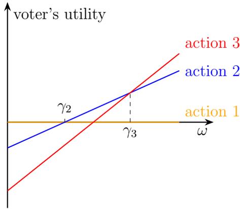
Consider an amendment voting setting where a voter chooses among three alternatives: maintaining the status quo (no bill, action 1); the amended bill (action 2); and the (unamended) bill (action 3).17 The state of the world is . The voter has linear preferences: her utility from action in state is given by . Moreover, and . Let and denote the cutoff states at which the voter is indifferent between actions 1 and 2, and actions 2 and 3, respectively:18 we impose . The voter's preferences are illustrated in Figure 6.
In this model, the voter's preferences over action are characterized by two parameters: , her reference point for action (her cardinal utility when the state is zero), and , her state sensitivity for action (how fast her cardinal utility increases in the state). The voter agrees that when the state is low (intermediate, high), action 1 (action 2, action 3, respectively) is optimal.
There is an expert who observes the state and discloses verifiable information to the voter (e.g., Jackson and Tan, 2013). The expert's preferences satisfy ; that is, the expert strictly prefers the bill to the amended bill, and the amended bill to no bill. This is a direct application of our model with and cutoffs , as defined above.19 The expert-preferred equilibrium is therefore characterized by Proposition 3.
Proposition 5 shows that the expert can be hurt if the voter becomes “more inclined toward” the bill in the sense that, all else equal, either the reference point or the state sensitivity for action 3 increases.
Proposition 5. If no commitment solution is implementable and at least one of the following happens:
- (i) the voter's state sensitivity for the bill, , increases,
- (ii) the voter's reference point for the bill, , increases,
then the expert's payoff in his preferred equilibrium may decrease.
When either (i) or (ii) occurs (or both), decreases. This implies that the expected state required to pass the bill is lowered, which benefits the expert directly: he can more frequently induce passage of the original bill. However, this also introduces an adverse indirect effect. Recall from the discussion after Proposition 3 that when no commitment solution is implementable, the upper bound of is pinned to by the binding revelation-proofness constraint. As falls, this constraint tightens, limiting the range of states over which the expert can credibly recommend action 2. The expert is therefore harmed when this indirect effect dominates the direct one. This may occur when the utility gap between the bill and the amended bill is smaller than that between the amended bill and the status quo (i.e., ), which is plausible in many voting scenarios.
6 Conclusion
This paper revisits a classic persuasion game (e.g., Milgrom, 1981) by changing one feature of the canonical model: the receiver has only finitely many actions. When the receiver can adjust her action finely, even a small improvement in beliefs leads to a better action for the sender, and the usual unraveling logic leaves little room for withholding information. With finitely many actions, by contrast, small changes in beliefs need not change the receiver’s action. This creates room for credible pooling even when the sender can prove any true fact, so full revelation is no longer the sole relevant equilibrium outcome. We show that the resulting set of equilibrium payoffs is organized by partitions of the state space with a simple geometric property—the laminar structure. Any sender-worst equilibrium is payoff equivalent to a fully revealing equilibrium, whereas a sender-preferred equilibrium often involves pooling nonadjacent states. We characterize such sender-preferred equilibria and use the characterization to compare sender-preferred equilibrium payoff with the commitment payoff: the payoff the sender would obtain if he could commit to an information structure, as in the information-design literature. This comparison identifies conditions under which the commitment payoff can be achieved in equilibrium.
The analysis yields broader lessons about disclosure and information design. The same environment can sustain a fully revealing equilibrium, a sender-preferred equilibrium with substantial pooling, and every payoff in between through simple laminar equilibria. This observation helps explain the variety of disclosure policies observed in practice and qualifies the welfare conclusions one can draw from the existence of a fully revealing equilibrium alone: observing that voluntary disclosure admits a fully revealing equilibrium does not imply that it delivers the receiver-preferred outcome; mandatory disclosure can still substantially improve receiver welfare by eliminating sender-preferred pooling. At the same time, our sufficient conditions for attaining the commitment payoff identify information-design problems for which the commitment assumption can be relaxed. On the other hand, if those conditions are met, the sender-preferred equilibrium and the equilibrium payoff set can be identified by solving the corresponding information-design problem. When the commitment payoff is unattainable, the sender-preferred equilibrium captures the trade-off between inducing actions more favorable to the sender and ensuring that no type wants to deviate by fully revealing the state.
A Omitted Proofs and Details
A.1 Proofs for Section 3
A.1.1 Preliminary characterization
In what follows, we employ the following result, which is essentially Theorem 1 in Titova and Zhang (2025) adapted to our setting.20 We provide a proof below for completeness.
Lemma 1. is an equilibrium partition if and only if it is obedient and revelation-proof.
Proof. Necessity is straightforward: if is not revelation-proof or obedient, then in every associated assessment, the sender has a profitable deviation to full revelation or the receiver is not best responding to an on-path message. For sufficiency, suppose that is an obedient and revelation-proof partition. Let be an associated assessment such that the receiver (1) has maximally skeptical off-path beliefs and (2) best responds according to her posterior mean and breaks ties in the sender-adversarial manner when indifferent. Specifically, for each , let , and if and , or and . Then, is an equilibrium, and thus is an equilibrium partition. Indeed, equilibrium conditions 2, 3, and 4 are satisfied by construction. Equilibrium condition 1 (the sender has no profitable deviations at each ) is satisfied because if and , then the sender's interim payoff is ; deviations to on-path messages with a higher index are not feasible, and deviations to on-path messages with a lower index or to off-path messages yield an interim payoff of at most . ■
A.1.2 Towards the proof of Theorem 1
To prove Theorem 1, we will need four auxiliary results.
Claim 1. Let be a mean-preserving contraction of with . Then there exist cutoffs with such that on for all and the inequality binds only at and .
Proof of Claim 1. First, let , where since and if . Since , is strictly increasing (since ), and is a step function, there exists such that for all . Since , we have , and hence the set
is nonempty. Let . If , then set and the proof is complete. For the rest of the proof, suppose that .
Observe that : if , then for all , which contradicts the definition of ; if , then for all , so that , a contradiction.
Next, we argue that . Suppose to the contrary that . Then, since is a CDF and hence right-continuous, there must exist such that for all , where the equality follows from the fact that is a step function. Then,
which contradicts the assumption that is a MPC of .
Now, let . Given that , , is strictly increasing, and is a step function, there exists such that for all . Consequently, implies that the set
is nonempty. Let . If , then set and the proof is complete. For the remainder of the proof, suppose that . Using the same steps as above, one can show that and . Proceeding inductively, one can find with such that . It must be that : suppose not, then because is strictly increasing, on ; but on the same interval, which implies that , a contradiction. Now set , the proof is complete. ■
Claim 2. If is a mean-preserving contraction of with , then it induces a laminar partition.
Proof. By Claim 1, on each of the intervals such that the MPC constraint only binds at the endpoints, the mass is redistributed to at most points, and there can be at most such intervals. We show that every such interval admits a laminar partition; the definition of a laminar partition then implies that the resulting partition is still laminar by taking the union.
Denote an arbitrary interval on which the MPC constraint only binds at the endpoints by ; that is, for all , and the inequality binds only at and .
The remainder of the proof is very similar to the proof of Lemma 11 in Candogan and Strack (2023), and hence we only provide an outline here; readers interested in details are directed to that paper. Let ; the proof proceeds by induction on . If , let ; then clearly where is a laminar partition of . If , let where ; then by Lemma 4 in Arieli et al. (2023), can be chosen such that and , which is laminar.
Taking as the base case, consider ; the induction hypothesis holds for . One can find a closed interval such that (i) , where is the probability mass function (pmf) of , and ,21 and (ii) . Consequently, conditional on , only has mass points, and Lemma 12 in Candogan and Strack (2023) shows that it is a MPC of . Invoking the inductive hypothesis, a laminar partition of , , is obtained, where . For every , let . Since is laminar, and for all , is also laminar. ■
Claim 3. Suppose that and such that and . Then, and .
Proof. We prove that ; the proof of is analogous. Since and , we have and .
Suppose, by contradiction, that . Then, , and . Furthermore,
a contradiction. Therefore, . ■
Claim 4. Let be an equilibrium. Define by
for all and . Then is also an equilibrium.
Proof. Equilibrium conditions 3 and 4 are unchanged because the sender's strategy and the belief system are identical to those in the original equilibrium. Condition 2 also remains true: if , then ; since is an equilibrium, must also satisfy condition 2.
It remains to verify condition 1. To simplify notation, for each message , let
Because the receiver is only indifferent between actions and when the expected state after seeing a message is exactly , for every message , is either a singleton or a pair of adjacent actions .
Define a function by . Because is strictly increasing in , is increasing. For every message we have : indeed, if , then and ; if , then and .
Now fix . Since is an equilibrium,
Because is increasing,
Therefore
so condition 1 also holds for . Thus, is an equilibrium.
A.1.3 Proof of Theorem 1
Proof of Part (a). First, observe that the fully revealing partition is obedient and revelation-proof since for each . By Lemma 1, it is an equilibrium partition. Next, we show that the sender's ex-ante payoff cannot be lower than in any other equilibrium. Let be the sender's payoff in state when the receiver knows the state and breaks ties in the sender-adversarial manner. By definition, . If the sender's ex-ante payoff is strictly below in an equilibrium, then his interim payoff is strictly below in a positive measure of states. Then, in each of those states, the sender has a profitable deviation toward sending message and receiving . Therefore, the sender's ex-ante payoff in a sender-worst equilibrium is exactly . This completes the proof of Part (a).
Proof of Part (b). We proceed in three steps. First, we show that if there exists a sender-preferred equilibrium, then there exists a sender-preferred laminar partitional equilibrium (Lemma 2). Second, we show that a sender-preferred laminar partitional equilibrium exists (Lemma 3). Third, we show that (Lemma 4).
Lemma 2. For any equilibrium in which the receiver plays pure strategy, there exists a laminar equilibrium partition that induces the same posterior mean distribution. Furthermore, if there exists a sender-preferred equilibrium, then there exists a sender-preferred laminar partitional equilibrium.
Proof of Lemma 2. Let be an equilibrium in which the receiver plays pure strategies. For any state in which the sender mixes, i.e., , since is an equilibrium, there exists such that for every . Thus, in every , there is an action played with probability 1 in this equilibrium. For every , let
By construction, , and for any . By Theorem 1(a) of Titova and Zhang (2025), for every , , and .
Consider the PMD with whose probability mass function is given by . By construction, is a mean-preserving contraction of the PMD induced by the equilibrium . Since the PMD induced by an equilibrium is itself a mean-preserving contraction of , is a mean-preserving contraction of with . Then by Claim 2, is also induced by a laminar partition with generic element . By construction, for every , , which implies obedience. Also by construction, for each .
We show next that is also revelation-proof, i.e., for all . Fix . Because is laminar, there exists such that for every action , ; and for every action , . This implies that is an interval. Let . Since for each , and , and since and for any , we have and . By Claim 3, we have , where the last inclusion follows since for all .
To prove the second statement, suppose that there exists a sender-preferred equilibrium. An immediate consequence of Claim 4 is that in a sender-preferred equilibrium, the receiver mixes on a null set of states. Therefore, we can focus on a sender-preferred equilibrium in which the receiver breaks ties in favor of the sender. Then by the first statement, there must exist a sender-preferred laminar equilibrium partition. ■
Lemma 3. Among all obedient and revelation-proof laminar partitions, there is one that maximizes the sender's ex-ante payoff.
Proof. The problem of finding a laminar partitional equilibrium that maximizes the sender's ex-ante payoff can be written as
To prove the lemma, it suffices to show that this problem has a solution, by Lemma 2.
Although an action may be never recommended, one can still assume that is nonempty by setting . Because is laminar, it is without loss of generality to assume that for each , is the union of at most intervals (cf. Observation 1). Consequently, adding singletons if necessary, one can always set as the union of exactly convex sets such that for all .
Let denote the set of closed, nonempty, and convex subsets of endowed with the Hausdorff distance; to simplify notation, we write henceforth. By Proposition 1 in Ely (2022), is compact; by Tychonoff's theorem, is compact in the product topology. The problem above can be transformed to
where the third constraint is equivalent to the conditional mean condition.
Define
We claim that is compact. To show this, it is enough to show that is a closed subset of . Take any that converges to in the product topology, then for each and . Consequently, because the limit of convergence in Hausdorff distance is preserved under finite unions,22 . Therefore, if , it must be that . Furthermore, if for all and , the same argument as the second paragraph in the proof of Lemma 2 in Ely (2022) shows that for all . Therefore, if for each and , it must be that . Thus, is a closed subset of .
Problem (5) is equivalent to
where constraint (7) supersedes the third constraint in problem (5) because for any , for all .
By the extreme value theorem, to show that a solution to problem (6) exists, it suffices to show that (i) the objective function is continuous, and (ii) the constraint set is nonempty and compact. Clearly, the constraint set is nonempty: for each , consider
then is feasible for this problem. Furthermore, by Proposition 1 in Ely (2022), is continuous on , and hence the objective is continuous.
Since is compact, to show that the constraint set is compact, it suffices to show that each of the constraints, (7) and (8), defines a closed subset of . Observe that if and with for all , then .23 Then because the limit of convergence in Hausdorff distance is preserved under finite unions, if for each , it must be that for each . Hence, (8) defines a closed subset of .
Next, we show that (7) does the same, which is equivalent to showing that if where for each , then
for all and implies that
for all . Because is continuous on , for all . Consequently, , and for each . Therefore, it only remains to show that
which is a consequence of being continuous on .
To prove this claim, we show that is both upper- and lower-semicontinuous. To see that it is upper-semicontinuous, pick any , and let ; we show that there exists such that for every , where is the -neighborhood of , . Because , there exist such that . The key observation here is that for any , it must be that . Then
where the inequality holds because . For small enough, since is absolutely continuous with respect to the Lebesgue measure,
Next, we show that is lower semicontinuous, that is, there exists such that for every , . Without loss of generality, assume . Consequently, is an interval of positive measure, and for any , . Then
where the inequality follows from the fact that on . Consequently, is both upper- and lower-semicontinuous, and hence continuous. This completes the proof.
Let denote a laminar partition associated with a sender-preferred equilibrium; by the previous two lemmas, such a partition exists. Denote the sender's ex-ante payoff from by .
Lemma 4. .
Proof. Let . Also, for each , let , and . It is easy to see that is a revelation-proof partition. Furthermore, for all by construction. Finally, the function is continuous at 0 and . Consequently, there exists sufficiently small such that , which makes an obedient partition. By Lemma 1, is an equilibrium partition; the sender's ex-ante payoff in that equilibrium is
which completes the proof.
Proof of Part (c). For any , we construct an obedient and revelation-proof laminar partition that yields by “blending” the fully informative partition and a sender-preferred laminar equilibrium partition (which exists by part (b)). For all ,
- for every such that , let ;
- if is such that , ;
- for every such that , let .
For any , and any , implies . Consequently, is obedient. It is also revelation-proof because both and are. Finally, because both and are laminar, it can be checked using (1) that is a laminar partition.
Let denote the sender's ex-ante payoff from : ; because , is continuous in . Since , by the intermediate value theorem, there exists such that . Thus, the partition is an obedient and revelation-proof laminar partition that yields .
A.1.4 Proof of Theorem 2
To establish Theorem 2, we first prove the following two preliminary results.
Claim 5. Let be a laminar partition associated with a sender-preferred equilibrium, and let . If , then for some .
Proof. Because is a laminar partition, must be an interval, and hence one can write . Furthermore, revelation proofness implies that .
To show that , it suffices to show that for all .24 Suppose not, so for some . The laminar structure implies that is the union of at most closed intervals; let be an interval such that and ; this interval is well-defined because is laminar and . Because and , for small enough , one can find such that
and
Now define a new partition with generic element by if , , and . is obedient by construction, and it is also revelation-proof because is; then by Lemma 1, is an equilibrium partition. Furthermore, it must be that : this is because by construction, and . Consequently, the sender's payoff is strictly higher in this new equilibrium since , which contradicts the assumption that is a partition associated with a sender-preferred equilibrium. ■
Claim 6. Let be a barely obedient laminar partition, and let be two unskipped actions with . Then if , then every and satisfy .
Proof of Claim 6. Because , either for every and , or for every and . The second possibility, however, cannot be true: by obedience, implies that , and . Consequently, , a contradiction. Therefore, it must be that for every and . ■
We are now ready to prove Theorem 2.
Proof of Theorem 2. We first show that must be barely obedient. Suppose to the contrary that , a laminar partition associated with a sender-preferred equilibrium, has for some non-null . By Lemma 1, is both obedient and revelation-proof. Let ; because , there exists with such that , and . Now consider the partition where , , and for . is obedient and revelation-proof because is, and the sender's ex-ante payoff from , , satisfies
a contradiction.
Next, we show that is the union of at most closed intervals for all . Recall that a laminar partition is defined by (1). Because must be an interval for all , is the union of at most intervals. By Claim 5, since is associated with a sender-preferred equilibrium, for all . Thus, for any , by taking out from , at most intervals are removed, and hence the remainder, namely , must be the union of at most intervals. By taking closure, is also the union of at most intervals.
Finally, we prove the equivalence between revelation proofness of a barely obedient laminar partition and the condition that for all unskipped such that either nests or is skipped. For convenience, for any , denote and .25
Suppose first that for all unskipped such that either nests or is skipped, and we show that for any action , . Since is laminar, it is without loss of generality to assume that if action is skipped, .
Now suppose is not skipped. There are two possibilities: either action is skipped or not. If is skipped, by assumption , implying . If instead is not skipped, there are two cases: either or not. If , then by assumption , implying that .
Suppose instead that is not a subset of , and suppose to the contrary that . Because is laminar, since is not a subset of (which means that does not nest ), it must be that . By Claim 6, for every and every , . This implies that for every , violating bare obedience, a contradiction. Thus, , which implies that .
For the other direction, we prove the contrapositive. If the condition is violated, that is, if for some unskipped such that either nests or is skipped, then is not a subset of . Thus, must violate revelation proofness. ■
A.2 Proofs and Details for Section 4
We first introduce the notion of a bi-pooling distribution.
Definition 4 (Bi-pooling distribution). A distribution is a bi-pooling distribution if there exists a collection of pairwise disjoint intervals such that
- for all , and ;26
- .
In particular, is called a pooling interval if , and it is called a bi-pooling interval if .
We call a bi-pooling distribution that solves the commitment problem (3) a bi-pooling solution.
The following observation is useful.
Lemma 5 (Candogan, 2019). Every bi-pooling solution to the commitment problem satisfies , where is such that for all .
An important consequence of Lemma 5 is that every signal realization can be identified by the action it induces. In particular, every induces the lowest unskipped action, and induces action for each . Moreover, if a bi-pooling solution is associated with a bi-pooling partition, then Lemma 5 implies that the partition must be barely obedient.
A.2.1 Proof of Theorem 3
By results in Kleiner et al. (2021) and Arieli et al. (2023), the commitment problem (3) admits a bi-pooling solution.
By Lemma 5, in any bi-pooling solution , if is nonempty but not a singleton, there must exist an interval on which action 1 is recommended, and is comprised of pooling intervals and/or bi-pooling intervals; in this case, can be viewed as a pooling interval. Otherwise, comprises pooling and/or bi-pooling intervals. The fact that every bi-pooling solution is associated with a bi-pooling partition therefore follows from Lemma 4 in Arieli et al. (2023): on every pooling interval, a single signal realizes, which induces a single action and hence ties to a single partitional element. On every bi-pooling interval , there exists such that one (deterministic) signal realizes when , and another signal realizes when , with the latter signal recommending a higher action. Then and correspond to two partitional elements and with , respectively. This observation and Lemma 5 together imply that the bi-pooling partition is barely obedient.
Fix a bi-pooling solution . To see that there is a unique barely obedient bi-pooling partition associated with it, we first note that every pooling interval necessarily ties to a unique partitional element. Hence, if a bi-pooling solution admits two distinct bi-pooling partitions, and , they must differ on a bi-pooling interval . Then there must exist and such that , , , and , with either , or , or both. Since and and are fixed, either , or , or both, a contradiction.
Finally, we show that the commitment solution is unique in generic communication environments. For any bi-pooling solution , let for each . If , set and ; otherwise, let and ; Lemma 5 then indicates that every bi-pooling solution is identified by . By Lemma D.1 in Candogan (2022), the condition that no three elements of the collection of points are collinear implies that any two bi-pooling solutions of problem (3) induce the same collection of . Then, because every bi-pooling solution is a mean-preserving spread of , any two such bi-pooling solutions must be identical. As noted in Kleiner et al. (2021) and Arieli et al. (2023), every extreme point of the set of solutions to problem (3) is a bi-pooling solution, and hence the solution to problem (3) must be a unique bi-pooling solution.
A.2.2 Proof of Proposition 1
Since the bi-pooling partition is barely obedient, the “if” direction follows from Lemma 1. For the other direction, suppose first that a bi-pooling solution is implementable. Since the commitment payoff is an upper bound on equilibrium payoffs, is the PMD induced by a sender-preferred equilibrium . By Theorem 3, is associated with a unique barely obedient bi-pooling partition ; an argument analogous to the one in the proof of Lemma 2 shows that is revelation-proof.
A.2.3 Proof of Proposition 2
We use the following result by Arieli et al. (2023) to prove Proposition 2. Say that is a feasible bi-pooling support for the interval (or just feasible for simplicity) if there exists a mean preserving contraction of whose support is .
Lemma 6 (Arieli et al., 2023). Fix an interval , and let satisfy . Then is feasible for the interval if and only if
- (i) , and
- (ii) .
Proof of Proposition 2. Suppose to the contrary that there exists a bi-pooling solution that is not implementable. Then by Corollary 1, the bi-pooling partition of , , must violate the condition therein. First suppose that there exists an unskipped action such that . There are two cases.
Case 1. is an interval; i.e., . There are two subcases:
(I) .
For , let solve . By Lemma 6, for close enough to , is feasible for . Consequently, the sender's payoff on , as a function of , is
where . To show that this is a profitable deviation, it suffices to show that . To this end, we first calculate
Letting , then , and
if and only if , and this is equivalent to
which is implied by (4).
(II) (and therefore ).
Define ; for small enough , is feasible for . Let denote the mean of ; note that . Then the sender's payoff as a function of on is
To show that this is a profitable deviation, it suffices to show that . Algebra reveals that
consequently, as ,
Because and by assumption, the sign of is the same as the sign of term in the square brackets in the right-hand side of (9). Thus, if and only if
Because , . Thus, (4) implies the inequality above.
Case 2. There is a partitional element with such that . In this case, , and . WLOG, assume that ; by Lemma 6, is feasible for , and
For , let solve . By (10) and Lemma 6, for close enough to , is feasible for . Consequently, one can find a profitable deviation similar to in Case 1 (I) mutatis mutandis.
Now suppose instead that there exists a pair of partitional elements and with , and . Since , this case is isomorphic to Case 1 when action is skipped. Hence, we can similarly find a profitable deviation.
Therefore, every bi-pooling solution must satisfy the condition in Corollary 1, and hence implementable. This completes the proof.
A.2.4 Proof of Corollary 2
By definition of , when is increasing, . Then since , it must be that . Now there are two cases. If , (4) must hold; then by Proposition 2, every bi-pooling solution can be implemented. If instead , it must be that ; this inequality and together imply (4). Again by Proposition 2, every bi-pooling solution can be implemented.
B Supplementary Appendix
This appendix is organized as follows:
- Section B.1 proves supplementary results for the special case in which the receiver has three actions.
- Section B.2 contains the proofs omitted from Appendix A.
- Section B.3 establishes the robustness of the set of partitional equilibria to two standard refinements: the never-a-weak-best-response (NWBR) criterion (Cho and Kreps, 1987) and the Grossman–Perry–Farrell refinement (Bertomeu and Cianciaruso, 2018).
B.1 Supplementary Results for Ternary Actions
In this section, we study the special case where the receiver has three actions: . Recall that is feasible for the interval if there exists a mean preserving contraction of whose support is .
Claim 7. If there does not exist such that is feasible for , then every bi-pooling solution is implementable.
Proof of Claim 7. By Lemma 6, is feasible for the interval if and only if
- (i) , and
- (ii) ,
where , and is such that . Then if there does not exist such that is feasible for , there are two cases:
- (a) (i) fails to hold for all ;
- (b) (i) holds for some , but (ii) fails for all such 's.
For Case (a), the only possibility is that . If this is the case, every bi-pooling solution has , and hence the unique bi-pooling partition has , and revelation proofness holds.
For Case (b), let us introduce some notation first. For each , if there exists such that , set ; otherwise let . Then for every , (i) holds. If (ii) fails for all such 's, it must be that . Note that this is not possible if : if this is the case, by definition, so it must be that , a contradiction. Consequently, in Case (b), (ii) must fail for , and hence every bi-pooling solution has , and . Thus, the unique bi-pooling partition associated with has and . Since by definition, revelation proofness must hold. This completes the proof.
Claim 8. All bi-pooling solutions to the information design problem are associated with the same bi-pooling partition.
Proof of Claim 8. It can be readily seen from the proof of Claim 7 that, if there does not exist such that is feasible for , then all bi-pooling solutions are associated with the same bi-pooling partition. Now suppose there exists such that is feasible for . Let denote the set of such 's; Lemma 6 implies that is a closed subset of . Consequently, the commitment payoff can be identified by the lower endpoint of the bi-pooling interval. Hence, each of them corresponds to a point in that maximizes the sender's ex-ante payoff (recall that ):
Taking derivative,
where
Consequently,
and its sign is determined by the terms between the squared brackets, which implies that is single-peaked in . Therefore, there must exist a unique that maximizes on . As a consequence, all bi-pooling solutions are associated with the same bi-pooling partition with , , and . ■
Claim 9. If no commitment solution is implementable, the sender-preferred laminar PE is such that , , and , where , and and are defined by
Furthermore,
Proof of Claim 9. By Theorem 2, if has nonempty interior, it must be that , and .27 Then to obtain the statement it suffices to show three things: (1) , namely has nonempty interior; (2) there exists such an ; and (3) there exists such a .
We show that has nonempty interior first. Suppose to the contrary that , then by Claim 7, there are two cases: , and for some . If , since the sender attains highest possible payoff in equilibrium, it must be that a commitment outcome is implementable, a contradiction. If instead for some , it must be that , as otherwise recommending action 2 on is a profitable deviation. Consequently, this bi-pooling partition is revelation-proof, and hence a commitment outcome is implementable, again a contradiction. Therefore, it must be that has nonempty interior.
To see that there exists such an , we first claim that . Suppose not, so
Without loss of generality, assume that there exists a bi-pooling solution features bi-pooled to for some .28 Consequently, there exist and with such that the (unique) bi-pooling partition associated with the bi-pooling solution is given by , , and . Then because and , we must have by (13). Thus, the bi-pooling solution must be implementable, a contradiction. As a consequence, it must be that ; it remains to show that . If instead , then . Consequently, it must be that and . This cannot be optimal: for any , define , and . Then for small enough, for each , and the sender's ex-ante payoff is strictly higher. Thus, it must be that .
To show that there exists such a , it suffices to show that . Suppose not, so . Let be small enough, and let be such that
Now define , and . Because the density is strictly positive, for small enough , , and . This creates a profitable deviation to the sender without violating revelation proofness.
Finally, to show that (12) must hold, suppose to the contrary that
An argument analogous to Case 1 (II) in the proof of Proposition 2 shows that the sender has a profitable deviation, and hence the bi-pooling partition with , , and cannot be associated with a sender-preferred laminar PE, a contradiction.
By Claim 9, the sender's ex-ante payoff in a sender-preferred equilibrium can be written as
where and are implicitly defined by the two equations in (11).
Claim 10. If no commitment outcome is implementable, the sender's ex-ante payoff in a sender-preferred equilibrium, , is increasing in .
Proof of Claim 10. Directly,
Using (11), by the implicit function theorem,
Plugging (15) and (16) into (14),
and we see that if and only if . Then since no commitment solution is implementable, by Claim 9, (12) implies that , and hence the sender's ex-ante payoff in a sender-preferred equilibrium is increasing in . ■
B.2 Remaining Omitted Proofs
B.2.1 Proof of Proposition 3
To solve for a sender-preferred equilibrium, we find a bi-pooling solution to the corresponding information design problem first, and check whether it is implementable using Corollary 1. If it is, a sender-preferred equilibrium is associated with a barely obedient bi-pooling partition that is also associated with the commitment solution.29
Now suppose that no commitment solution is implementable. By Theorem 2, there exist , , and such that , and .30 By Claim 9, there exist and such that
Consequently, and can be implicitly defined as functions of , and hence the sender's ex-ante payoff can be parametrized by , so long as :
By Claim 10, is increasing in . Hence, the partition corresponding to the sender's preferred equilibrium can be found by setting , which yields the expression in the statement of the claim.
B.2.2 Proof of Corollary 3
Recall that and is normalized to zero; hence when , Equation (4) in the main text reduces to
And because , the right-hand side of (17) further reduces to . Then since is increasing, ; thus, if , or , (17) must hold. Consequently, by Proposition 2, every bi-pooling solution can be implemented. By Claim 7, all bi-pooling solutions induce the same bi-pooling partition. Then because the set of bi-pooling solutions is the set of extreme points of the solution correspondence of the information design problem, all commitment solutions must be associated with the same bi-pooling partition. Thus, every commitment outcome is implementable.
B.2.3 Proof of Proposition 4
Let denote the cutoff quality that the buyer is indifferent between purchasing and units: it solves
so . Letting and , the buyer buys units of the product if and only if . If , is strictly decreasing in , and thus
is strictly decreasing in . Since the seller's gain from the buyer purchasing one more unit is , Proposition 4 follows from Corollary 3.
B.2.4 Proof of Proposition 5
If either increases, or increases, or both, decreases. By Proposition 3, when no commitment outcome can be implemented, the sender's ex-ante payoff is given by
where and are implicitly defined by
Now
By the implicit function theorem,
Plug (19) and (20) into (18),
whose sign is determined by
By Claim 9, if no comment outcome is implementable, it must be that . Consequently, the sign of the second term of (21) must be positive, and the first term has a strictly negative sign. Hence as decreases, the expert's ex-ante payoff in her preferred equilibrium strictly decreases if the second term is larger in absolute value, which establishes the statement.
B.3 Equilibrium Refinement
It is natural to ask whether the equilibria of the disclosure game considered in this paper are credible in that they survive certain equilibrium refinements. We consider the following two equilibrium refinements:
- The Never-a-Weak-Best-Response (NWBR) Criterion, proposed by Cho and Kreps (1987), is a strengthening of a few equilibrium refinements that are extensively used in the literature, which includes the Intuitive Criterion, D1, and D2.31
- The Grossman-Perry-Farrell equilibrium, proposed by Bertomeu and Cianciaruso (2018), is based on the perfect sequential equilibrium of Grossman and Perry (1986) and neologism-proofness of Farrell (1993).
It can be shown that every PE of the disclosure game we study is a Grossman-Perry-Farrell equilibrium, and every PE outcome survives the NWBR Criterion. We use the term “type” instead of “state” henceforth to ease exposition.
B.3.1 Never-a-Weak-Best-Response (NWBR) Criterion
We introduce some notation first. For any , let denote the set of all mixed strategy best responses for the receiver to message for any belief .32 Moreover, let denote the equilibrium payoff of type . Finally, for any equilibrium and an off-path message , define
and
in words, is the set of mixed strategy best responses that make type strictly prefer to her equilibrium message, and is the set of mixed strategy best responses that make type exactly indifferent.
Definition 5. An equilibrium survives the NWBR criterion if for every and any , implies that .
Claim 11. For every PE , there exists such that survives the NWBR criterion.
Proof. Fix a PE , and let denote the associated partition. For every , let . Let be such that for all , and for any , let
By the definition of PE, the receiver never mixes on path, and hence for any , if and only if , where is the Dirac measure at action . Furthermore, define
then the lowest action in is . Now for any ,
Then if and only if with , which is in turn equivalent to . Then (22) implies that . Consequently, survives the NWBR criterion. ■
B.3.2 Grossman-Perry-Farrell Equilibrium
Definition 6. Fix a PE . Say that is a self-signaling set if33
An PE is a Grossman-Perry-Farrell equilibrium if there does not exist a self-signaling set.
Claim 12. Every PE is a Grossman-Perry-Farrell equilibrium.
Proof. Fix a PE , and let denote the associated partition. Suppose there exists a self-signaling set . Let
Because is a self-signaling set, it must be that . But then revelation proofness of implies that there must exist such that with , a contradiction. ■
References
-
ALI, S. N., A. KLEINER, AND K. ZHANG (2024): “From Design to Disclosure,” Working paper.
-
ARIELI, I., Y. BABICHENKO, R. SMORODINSKY, AND T. YAMASHITA (2023): “Optimal persuasion via bi-pooling,” Theoretical Economics, 18, 15–36.
-
ARIELI, I. AND C. STEWART (2025): “Bayesian Persuasion without Commitment,” Working paper.
-
BEDERSON, B. B., G. Z. JIN, P. LESLIE, A. J. QUINN, AND B. ZOU (2018): “Incomplete Disclosure: Evidence of Signaling and Countersignaling,” American Economic Journal: Microeconomics, 10, 41–66.
-
BEN-PORATH, E., E. DEKEL, AND B. L. LIPMAN (2025): “Evidence in Games and Mechanisms,” Annual Review of Economics, forthcoming.
-
BERTOMEU, J. AND D. CIANCIARUSO (2018): “Verifiable disclosure,” Economic Theory, 65, 1011–1044.
-
BEST, J. AND D. QUIGLEY (2024): “Persuasion for the long run,” Journal of Political Economy, 132, 1740–1791.
-
CANDOGAN, O. (2019): “Optimality of Double Intervals in Persuasion: A Convex Programming Framework,” Working paper.
-
(2022): “Persuasion in Networks: Public Signals and Cores,” Operations Research, 70, 2264–2298.
-
CANDOGAN, O. AND P. STRACK (2023): “Optimal Disclosure of Information to Privately Informed Agents,” Theoretical Economics, 18, 1225–1269.
-
CHO, I.-K. AND D. M. KREPS (1987): “Signaling Games and Stable Equilibria,” The Quarterly Journal of Economics, 102, 179–221.
-
DAI, Y., D. FUDENBERG, AND H. PEI (2026): “Bayesian Persuasion with Selective Disclosure,” Working paper.
-
DRANOVE, D. AND G. Z. JIN (2010): “Quality Disclosure and Certification: Theory and Practice,” Journal of Economic Literature, 48, 935–963.
-
ELY, J. C. (2022): “A Cake-Cutting Solution to Gerrymandering,” Working paper.
-
ENELOW, J. M. (1981): “Saving Amendments, Killer Amendments, and an Expected Utility Theory of Sophisticated Voting,” The Journal of Politics, 43, 1062–1089.
-
ENELOW, J. M. AND D. H. KOEHLER (1980): “The Amendment in Legislative Strategy: Sophisticated Voting in the U.S. Congress,” The Journal of Politics, 42, 396–413.
-
FARRELL, J. (1993): “Meaning and Credibility in Cheap-Talk Games,” Games and Economic Behavior, 5, 514–531.
-
FELTOVICH, N., R. HARBAUGH, AND T. TO (2002): “Too Cool for School? Signalling and Countersignalling,” RAND Journal of Economics, 33, 630–649.
-
FUDENBERG, D. AND J. TIROLE (1991): Game Theory, MIT Press.
-
GENTZKOW, M. AND E. KAMENICA (2016): “A Rothschild-Stiglitz Approach to Bayesian Persuasion,” American Economic Review: Papers & Proceedings, 106, 597–601.
-
GIECZEWSKI, G. AND M. TITOVA (2025): “Coalition-Proof Disclosure,” Working paper.
-
GIOVANNONI, F. AND D. J. SEIDMANN (2007): “Secrecy, Two-sided Bias and the Value of Evidence,” Games and Economic Behavior, 59, 296–315.
-
GROSSMAN, S. J. (1981): “The Informational Role of Warranties and Private Disclosure about Product Quality,” Journal of Law and Economics, 24, 380–391.
-
GROSSMAN, S. J. AND O. D. HART (1980): “Disclosure Laws and Takeover Bids,” The Journal of Finance, 35, 323–334.
-
GROSSMAN, S. J. AND M. PERRY (1986): “Perfect Sequential Equilibrium,” Journal of Economic Theory, 39, 97–119.
-
GUO, Y. AND E. SHMAYA (2019): “The interval structure of optimal disclosure,” Econometrica, 87, 653–675.
-
(2021): “Costly miscalibration,” Theoretical Economics, 16, 477–506.
-
HARBAUGH, R. AND T. TO (2020): “False Modesty: When Disclosing Good News Looks Bad,” Journal of Mathematical Economics, 87, 43–55.
-
JACKSON, M. O. AND X. TAN (2013): “Deliberation, Disclosure of Information, and Voting,” Journal of Economic Theory, 148, 2–30.
-
KLEINER, A., B. MOLDOVANU, AND P. STRACK (2021): “Extreme Points and Majorization: Economic Applications,” Econometrica, 89, 1557–1593.
-
KOESSLER, F. AND V. SKRETA (2023): “Informed information design,” Journal of Political Economy, 131, 3186–3232.
-
KOHLBERG, E. AND J.-F. MERTENS (1986): “On the Strategic Stability of Equilibria,” Econometrica, 54, 1003–1037.
-
KOLOTLIN, A. (2018): “Optimal Information Disclosure: A Linear Programming Approach,” Theoretical Economics, 13, 607–635.
-
KUVALEKAR, A., E. LIPNOWSKI, AND J. RAMOS (2022): “Goodwill in Communication,” Journal of Economic Theory, 203, 105467.
-
LIN, X. AND C. LIU (2024): “Credible persuasion,” Journal of Political Economy, 132, 2228–2273.
-
LIPNOWSKI, E. (2020): “Equivalence of Cheap Talk and Bayesian Persuasion in a Finite Continuous Model,” Working paper.
-
LIPNOWSKI, E. AND D. RAVID (2020): “Cheap Talk With Transparent Motives,” Econometrica, 88, 1631–1660.
-
LIPNOWSKI, E., D. RAVID, AND D. SHISHKIN (2022): “Persuasion via Weak Institutions,” Journal of Political Economy, 130, 2705–2730.
-
(2025): “Perfect Bayesian Persuasion,” Journal of Political Economic Microeconomics, forthcoming.
-
MATHEVET, L., D. PEARCE, AND E. STACCHETTI (2022): “Reputation and Information Design,” Working paper.
-
MCLENNAN, A. (2018): Advanced Fixed Point Theory for Economics, vol. 25, Springer.
-
MILGROM, P. (2008): “What the Seller Won’t Tell You: Persuasion and Disclosure in Markets,” Journal of Economic Perspectives, 22, 115–131.
-
MILGROM, P. R. (1981): “Good News and Bad News: Representation Theorems and Applications,” Bell Journal of Economics, 12, 380–391.
-
MIN, D. (2021): “Bayesian Persuasion under Partial Commitment,” Economic Theory, 72, 743–764.
-
NGUYEN, A. AND T. Y. TAN (2021): “Bayesian Persuasion with Costly Messages,” Journal of Economic Theory, 193, 105212.
-
PEI, H. (2023): “Repeated Communication with Private Lying Costs,” Journal of Economic Theory, 210, 105668.
-
PEREZ-RICHET, E. (2014): “Interim Bayesian Persuasion: First Steps,” American Economic Review, 104, 469–474.
-
TITOVA, M. AND K. ZHANG (2025): “Persuasion with verifiable information,” Journal of Economic Theory, 230, 106102.
-
ZAPECHELNYUK, A. (2023): “On the Equivalence of Information Design by Uninformed and Informed Principals,” Economic Theory, 76, 1051–1067.