Targeted Advertising in Elections
American Economic Journal: Microeconomics, Forthcoming, 2026
How does targeted advertising influence electoral outcomes? This paper presents a one-dimensional spatial model of voting in which a privately informed challenger persuades voters to support him over the status quo. I show that targeted advertising enables the challenger to persuade voters with opposing preferences and swing elections decided by such voters; under simple majority, the challenger can defeat the status quo even when it is located at the median voter's bliss point. Ex-ante commitment power is unnecessary—the challenger succeeds by strategically revealing different pieces of verifiable information to different voters. Publicizing all political ads would mitigate the negative effects of targeted advertising and help voters collectively make the right choice.
@article{TA-elections,
  author = {Maria Titova},
  title = {Targeted Advertising in Elections},
  journal = {American Economic Journal: Microeconomics},
  volume = {Forthcoming},
  year = {2026},
  doi = {10.1257/mic.20240479},
  url = {https://www.aeaweb.org/articles?id=10.1257/mic.20240479},
}
Abstract
How does targeted advertising influence electoral outcomes? This paper presents a one-dimensional spatial model of voting in which a privately informed challenger persuades voters to support him over the status quo. I show that targeted advertising enables the challenger to persuade voters with opposing preferences and swing elections decided by such voters; under simple majority, the challenger can defeat the status quo even when it is located at the median voter's bliss point. Ex-ante commitment power is unnecessary—the challenger succeeds by strategically revealing different pieces of verifiable information to different voters. Publicizing all political ads would mitigate the negative effects of targeted advertising and help voters collectively make the right choice.
KEYWORDS: Persuasion, verifiable information, targeted advertising, elections
JEL CLASSIFICATION: D72, D82, D83
1. Introduction
Targeted advertising, broadly defined as private messaging aimed at specific groups of voters, played a key role in many successful electoral campaigns. In 1960, John F. Kennedy’s campaign distributed two million copies of “the blue bomb”—a pamphlet advertising his support of civil rights—to African American churches across the U.S. Decades later, George W. Bush’s 2004 reelection campaign used direct mail to communicate his opposition to gay marriage and support for “traditional family values” to evangelical Christian households. More recently, the 2016 Brexit referendum and the Trump presidential campaign both employed the services of Cambridge Analytica, a data mining firm, to design and distribute thousands of targeted ads to diverse audiences. Although these examples suggest broad awareness of a correlation between targeted advertising and electoral success, the precise mechanisms by which tailoring messages to different voters influences election outcomes remain poorly understood.
This paper proposes a simple theoretical model that fills this gap. The model is grounded in three stylized facts about electoral campaigns. First, voters have incomplete information and update their beliefs in response to campaign messages (Kendall, Nannicini, and Trebbi, 2015; Spenkuch and Toniatti, 2018; Le Pennec and Pons, 2023). Second, politicians use the strategy of ambiguity to avoid making precise statements about their positions on issues (Page, 1978; Druckman, Kifer, and Parkin, 2009; Fowler et al., 2021). Third, politicians tailor messages to specific groups of voters (Hillygus and Shields, 2014). I identify a novel mechanism by which targeted advertising changes electoral outcomes. In particular, I show that privately revealing different pieces of information to different voters allows politicians to persuade voters with diametrically opposing preferences and win otherwise unwinnable elections, in which such voters are pivotal.
My model has two components: an advertising campaign followed by an election.1 In the election, a unit mass of voters chooses between two options, the challenger and the status quo. Voters care about the candidates’ policy outcomes, which represent proposed policies, their implementation, or welfare consequences. The challenger’s policy outcome is initially unknown to the voters, while the status quo policy outcome is com-monly known and normalized to zero. Voters have single-peaked and single-crossing preferences, with the leading example being quadratic loss.2 The goal of the office-motivated challenger is to convince a decisive coalition of voters to approve his proposal. I model the challenger's advertising campaign as a game of persuasion with verifiable information (Grossman and Hart, 1980, Milgrom, 1981 and Grossman, 1981). That is, I assume that the challenger privately knows his policy outcome and can send any subset of that contains . Conceptually, this communication protocol allows the challenger to lie by omission but not commission: a message informs a voter that the challenger's policy outcome is moderately left, but is only partially informative because could be anywhere between and . Communication with verifiable information is a reasonable middle ground between the possibilities identified by Persson and Tabellini (2002), who famously wrote (p. 483), "It is thus somewhat schizophrenic to study either extreme: where promises have no meaning or where they are all that matter." I consider two versions of the game: public advertising and targeted advertising. The former models a public advertising campaign in which the challenger sends the same message to all voters. The latter models a targeted advertising campaign in which the challenger knows the voters' bliss points and sends private messages to different groups of voters.
The main contribution of the paper is showing that targeted advertising allows the challenger to win elections that are unwinable with public advertising.3 My first two results (Theorems 1 and 2) characterize elections (described by a set of voters' bliss points and a set of decisive coalitions) that are unwinable for the challenger with public and targeted advertising, respectively. Theorem 1 states that an election is unwinable for the challenger with public advertising if and only if there is no decisive coalition of left or right voters. The intuition is simple: if there is a decisive coalition of left (right) voters, then the challenger can use a fully revealing strategy and win when his policy outcome is left (right) of the status quo. Otherwise, all decisive coalitions include status quo voters (whose bliss point is the status quo) or left and right voters (who have diametrically opposing preferences, so the status quo is already the best compromise). Theorem 2 states that an election is unwinable for the challenger with targeted advertising if and only if every decisive coalition includes a status quo voter. In particular, targeted advertising makes it possible for the challenger to convince voters on the opposite sides of the status quo with a positive probability by telling them different things. Under simple majority, Theorems 1 and 2 classify elections as follows:
- I. If the median voter's bliss point is left or right of the status quo, then the election is winnable with public advertising.
- II. If the median voter's bliss point is at the status quo, but status quo voters do not form a majority, then the election is unwinable with public advertising but winnable with targeted advertising.
- III. If the median voter's bliss point is at the status quo and status quo voters do form a majority, then the election is unwinable with public or targeted advertising.
The second part of the paper focuses on the optimal targeted advertising strategy that maximizes the challenger's (ex-ante) odds of winning elections that are unwinable with public advertising. I make a further simplification that all left voters have the same bliss point and all right voters have the same bliss point . Below I use a motivating example in which , , the voters' preferences are quadratic, the minimal decisive coalition includes left and right voters, and , to illustrate the following two results: Proposition 2 identifies the optimal targeted advertising strategy, while Proposition 3 describes the comparative statics as the right voters become more extreme/the electorate becomes more polarized.
Consider the following strategy of the challenger: to the left voters, he reveals whether his policy outcome is in the set , or not.4 To the right voters, he reveals whether his policy outcome is in , or not. When a left voter receives message , she learns that the challenger's policy outcome could be anywhere in , which is just enough information to convince her to approve.5 By similar reasoning, a right voter is convinced after message . This strategy leads to the following electoral outcome: the left voters approve if and only if and the right voters approve if and only if . Given that left and right voters form a decisive coalition, the challenger wins the election if and only if his policy outcome is between and . His ex-ante odds of winning are 30% – a massive improvement over his odds of winning without targeted advertising, which are 0%. Proposition 2 confirms that the described electoral outcome is an equilibrium outcome with the highest odds of the challenger winning across all equilibria of the targeted advertising game.

To see how this challenger-preferred equilibrium outcome changes as right voters become more extreme, suppose the right voters' bliss point increases from to . Following the same logic as above, we find that the convincing messages are for left voters and for right voters. The challenger wins when his policy outcome is between and , exactly as before. However, the challenger's equilibrium odds of winning may be even higher. Specifically, observe that when the challenger's policy outcome is between and , the strategy described above convinces right but not left voters. However, left voters actually prefer policy outcomes in to those in as the former are closer to their bliss point. Hence, we can recalculate the message that convinces left voters (making them indifferent between approval and rejection), forcing it to start at . That message is . Figure 2 illustrates the electoral outcome after right voters become more extreme.

In the new equilibrium, the set of winning policy outcomes is and the challenger's odds of winning are 33.96%. Proposition 3 confirms that when right voters become more extreme, the set of winning policy outcomes shifts in the opposite direction, to the left; also, the challenger's odds of winning increase. Intuitively, when right voters become more extreme, their dissatisfaction with the status quo grows, which makes them persuadable by wider ranges of policy outcomes.
My findings suggest a novel explanation for why politicians use the strategy of ambiguity: advertising different ranges of policy outcomes to different voters allows politicians to persuade voters with diametrically opposing preferences without lying (by commission) to any of them. Previous explanations for why politicians use the strategy of ambiguity include voters' risk-seeking behavior (Shepsle, 1972), candidates' preference for ambiguity (Aragonès and Neeman, 2000), subsequent elections (Meirowitz, 2005, Alesina and Holden, 2008), resolution of uncertainty after an election (Kartik, Van Weelden, and Walton, 2017). Two previous papers find that ambiguity enables politicians to persuade voters with opposing preferences: in Callander and Wilson (2008), voters have context-dependent preferences, and in Tolvanen (2024), the voters' preferences are correlated with the state of the world. I reach a similar conclusion in a setting where voters have standard single-peaked and single-crossing preferences.
This paper builds on the literature comparing public and private communication in both electoral environments and broader sender-receiver settings. When messages are verifiable (like in this paper) and candidates are symmetric, unraveling occurs: competing politicians voluntarily disclose all information, whether advertising is public or private (Janssen and Teteryatnikova, 2017; Schipper and Woo, 2019). However, I show that when candidates are asymmetric—specifically, when only the challenger advertises privately—there are equilibria without unraveling, and the challenger generally prefers private to public communication with verifiable information. In cheap-talk models, by contrast, senders often favor public communication because it limits the number of possible deviations in each state of the world (Farrell and Gibbons, 1989, Koessler, 2008, Goltzman and Pavlov, 2011, Bar-Isaac and Deb, 2014).6 Consequently, targeted advertising cannot swing unwinnable elections if ads consist only of cheap talk. My analysis thus highlights that persuading voters with opposing preferences requires providing selective evidence or easily verifiable facts. Finally, in the information-design literature, the sender has ex-ante commitment power and generally prefers private communication (Arieli and Babichenko, 2019, Chan et al., 2019, Heese and Lauermann, 2025). That said, public and private information design yield the same outcomes if receivers possess private information and choose between two actions (Kolotilin et al., 2017), if receivers compete (Asseyer and Ravindran, 2025), and in elections with unanimity voting (Bardhi and Guo, 2018). Since the challenger-preferred equilibrium strategy described in Proposition 2 is also an information design solution, my analysis identifies an electoral environment in which the sender strictly prefers private to public information design.
My analysis suggests that targeted advertising is bad for democracy because it elects politicians who are guaranteed to lose when voters possess the same information. For example, under simple majority, targeted advertising allows the challenger to beat the status quo located at the median voter's bliss point, which, according to various versions of the median voter theorem, is unbeatable. The most effective policy to make targeted advertising obsolete is to publicize all ads transmitted during electoral campaigns. While voters may still make mistakes due to incomplete (but public) information, having a common belief would be sufficient for them to collectively make the right choice.
2. Model
There is a challenger (he/him) and a unit mass of voters (she/her). The space of policy outcomes is . Let , where , denote the ordered set of voters' bliss points; I will refer to as the electorate.7 I refer to a voter with bliss point as "voter " when there is no possibility of confusion. The game proceeds as follows.
-
The challenger learns his policy outcome , drawn from a common prior distribution that has full support and no atoms.8
-
The challenger sends messages to voters. Each message is a Borel subset of (a statement about his policy outcome) that contains a grain of truth, . This communication protocol, introduced by Grossman and Hart (1980), Milgrom (1981), and Grossman (1981), allows the challenger to lie by omission and send messages that contain policy outcomes other than . However, it does not allow the challenger to lie by commission and send messages that do not include . I consider two versions of the game:
- targeted advertising: the challenger chooses a collection of private messages , and voters with bliss point observe message only;
- public advertising: the challenger chooses a public message that is the same for all .
- Each voter decides whether to approve the challenger's policy outcome or reject it in favor of the status quo. I normalize the status quo policy outcome to 0.
- Payoffs are realized. The outcome of the vote is determined by a voting rule that, for any profile of voters' approve/reject decisions, specifies whether the challenger wins (and receives a payoff of 1) or loses (and gets 0). I say that a coalition of voters is decisive if the challenger (i) wins whenever all voters in approve and (ii) loses whenever all voters in reject.9 I let denote the set of decisive coalitions. By construction, is monotonic ( and imply ) and proper ( implies ).10 I assume that is nonempty (equivalently, ) and refer to the pair as the election.
Voters are expressive, meaning that the payoff of voter depends on the policy outcome that she votes for (which is if she approves, and 0 if she rejects).11 I describe voter 's preferences using her net payoff from approval, , so that weakly prefers to approve whenever . I let voter 's approval set be the set of policy outcomes that she prefers to approve under complete information.
I assume that is continuous, measurable, bounded, and satisfies two properties standard in spatial voting models:
ASSUMPTION 1. Voters' preferences are single-peaked (strictly quasiconcave): for each voter , her net payoff from approval is strictly increasing on and strictly decreasing on .
One relevant consequence of Assumption 1 is that voter 's upper contour sets are convex. In particular, the approval set is an interval for left voters with , a point for status quo voters with , and an interval for right voters with .
ASSUMPTION 2. Voters' preferences are single-crossing: for each belief ,
and
I refer to Assumption 2 as a single-crossing property because it states that the sign of is monotone in for all .12 Assumption 2 has two consequences relevant to our analysis. (SC1) states that if a left voter prefers to approve, then all right voters prefer to reject, and vice versa. (SC2), on the other hand, states that if a left (right) voter prefers to approve, then all left (right) voters with bliss points further away from the status quo also prefer to approve. For convenience, I refer to such voters as more extreme:
DEFINITION 1. A left voter is more extreme than a left voter if . A right voter is more extreme than a right voter if .
I illustrate my results for quadratic voter preferences, , which is one example of standard preferences that satisfy all the assumptions.
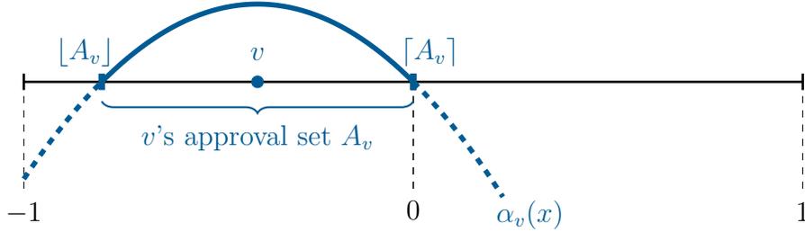
Figure 3 illustrates the preferences of a quadratic voter .
I focus on weak perfect Bayesian equilibria in which the voters' inference is consistent with disclosure on and off the path. In equilibrium, (i) the challenger sends messages that maximize his expected payoff; (ii) each voter approves whenever her expected net payoff from approval is non-negative under her posterior belief; (iii) each voter calculates her posterior using Bayes' rule on the equilibrium path; and (iv) a voter's posterior belief after an off-path message is an element of . I restrict attention to equilibria in which all voters with bliss point act the same. For ease of exposition, I also assume that status quo voters always reject.13 I denote the challenger's interim expected utility—i.e., the probability that he wins the election when his policy outcome is —by . I refer to the challenger's ex-ante utility as his odds of winning.
I say that a set of policy outcomes is implementable if there exists an equilibrium in which the challenger's interim utility is . In that equilibrium, the challenger wins if and only if (i.e., is the set of “winning” policy outcomes) and his odds of winning are .
Most of my constructive results involve equilibria in which the challenger uses a simple pure strategy of revealing whether his policy outcome is or is not in some set. Let be a collection of subsets of . A direct strategy is defined as . In words, when the challenger's policy outcome is , he tells voter whether (by sending message ) or not (by sending message ). A direct public strategy is one with for all . When the challenger uses a direct strategy, voter hears one of two on-path messages, , and thus learns whether and nothing else; her posterior belief is then . I say that voter is willing to approve a set of policy outcomes (if the challenger uses a direct strategy and receives message ) if it satisfies her obedience constraint:
3. Analysis
To begin analysis, let us first classify elections in the following way. I say that coalition of voters is left (right), denoted (), if it consists of left (right) voters only; I say that is a mixed coalition if it has both left and right voters.
DEFINITION 2. An election is a
-
left- (right-) leaning election if there exists a left (right) decisive coalition;
-
status quo-leaning election if every decisive coalition includes a status quo voter;
-
polarized election if there exists a mixed decisive coalition and there are no left or right decisive coalitions.
This classification is exhaustive: every election belongs to exactly one category.14
Given a coalition of voters , let and be its left pivot and right pivot, if they exist, respectively. Let us define a representative voter as the voter whose approval set equals the union of the approval sets of all decisive coalitions.
DEFINITION 3. The representative voter of election is the voter such that .
Voter essentially represents the preferences of the entire electorate because, under complete information, if she prefers to approve, then so does at least one decisive coalition, and if she prefers to reject, then so do all decisive coalitions. The lemma below determines the location of the representative voter in each election type, allowing us to state subsequent results for the public advertising game in terms of a single voter rather than sets of decisive coalitions.
LEMMA 1. Consider an election . Then,
Proof. Recall that from Assumption 1, the approval set of voter is if , if , and if . Therefore, for any decisive coalition that is mixed or includes a status quo, we have . Consequently, for status quo-leaning and polarized elections, we have .
Next, observe that from (SC2), if voter is less extreme than voter , then . Then, for any left coalition , we have , because is the least extreme voter in . Therefore, for any left-leaning election , we have
where . The proof is analogous for a right-leaning election. ■
Public Advertising
In the public advertising game, the voters' common prior belief is updated to a common posterior. Therefore, the electorate faces a collective choice problem: whether to choose a safe option (the status quo) or a lottery over the challenger's policy outcomes (represented by their common posterior belief ). The first result describes which elections are "unwinnable" for the challenger with public advertising.
THEOREM 1. In the public advertising game,
- The challenger's odds of winning are zero in every equilibrium if and only if the election is status quo-leaning or polarized, i.e., there is no left or right decisive coalition.
- A set of policy outcomes is implementable in a left/right-leaning election if it is obedient for the representative voter and includes her approval set.
As the equilibrium constructions from the proofs of Theorems 1 and 2 are used later in Section 4, I provide the proofs of these theorems in the main text.
Proof. I prove sufficiency of part 1 directly. If there is no left or right decisive coalition, then the election is either status quo-leaning or polarized. In both cases, the challenger convinces a decisive coalition only if the public belief is , or whenever , which has zero prior measure. To see this, observe that for any belief other than , status quo voters strictly prefer to reject; also, left and right voters never prefer to approve at the same time by SC1. Therefore, the challenger's odds of winning are zero in every equilibrium of the public advertising game unless there is a left or right decisive coalition.
To prove the rest of the theorem, we consider (without loss) a left-leaning election with representative voter and construct an equilibrium that implements , where and . Note that such exists—for example, we can let .
Suppose that the challenger uses the direct public strategy . When message is heard on the path, the public posterior becomes ; the representative voter prefers to approve because satisfies her obedience constraint. Since is the least extreme voter in some left decisive coalition , by (SC2) we have for all , which means that the entire decisive coalition prefers to approve after message .
We now show that when the public posterior is supported on (for instance, after message ), the challenger loses the election because every decisive coalition includes a voter who strictly prefers to reject. First, voter strictly prefers to reject. Indeed, since , we have for all , and therefore . Next, all left voters less extreme than also strictly prefer to reject: by the contrapositive of (SC2), implies for all . In the left-leaning election under consideration, every decisive coalition is left, mixed, or includes a status quo voter. Every left decisive coalition includes a voter by Lemma 1. Every other decisive coalition contains a voter who strictly prefers to reject by the argument in the first paragraph of this proof. Consequently, the challenger loses whenever the public belief is supported on (in particular, when message is heard on the path). Therefore, if the challenger uses strategy , he wins if and only if , his interim utility is , and his odds of winning are .
Finally, we specify the voters' off-path beliefs and show that the challenger does not have profitable deviations. When , the challenger receives the highest possible payoff and, therefore, has no profitable deviations. We thus do not restrict voters' beliefs for off-path messages . Conversely, when the challenger's policy outcome is not in , his on-path payoff is zero; a profitable deviation would require sending a message that results in a win. To deter such deviations, we require voters to hold skeptical beliefs. Specifically, for any off-path message , we restrict the voters' posterior to be an element of . This ensures that any message that the challenger can send when induces a public posterior supported on , after which the challenger loses the election, as shown in the previous paragraph. This completes the equilibrium characterization and the proof.
Theorem 1 essentially states that an election is winnable with public advertising if and only if the representative voter is left or right. Furthermore, in winnable elections, the challenger effectively caters to the representative voter: a set of “winning” policy outcomes is implementable if it contains that voter’s approval set and satisfies her obedience constraint. The former condition ensures that the representative voter (and thus some voter in every decisive coalition) strictly prefers to reject after every message available to the challenger when . The latter condition guarantees that the representative voter (and thus every voter in some decisive coalition) approves after message . In Section 4, we will characterize the largest implementable set of winning policy outcomes for a left-leaning election in which all voters’ bliss points are the same.
Under simple majority, we arrive at a familiar characterization of elections that are unwinnable with public advertising.
COROLLARY 1. Under simple majority, the challenger’s odds of winning are zero in every equilibrium of the public advertising game if and only if the status quo is the median voter’s bliss point.
The proof of the corollary is straightforward: if there is no left or right decisive coalition, then the status quo is the median voter’s bliss point. Note that Corollary 1 is a special case of median voter theorems for collective choice problems under uncertainty, which state that the median voter’s bliss point defeats any lottery, degenerate or nondegenerate. The median voter theorem holds for single-peaked and strictly concave voter preferences (Shepsle, 1972), and those that have single-crossing expectational differences (Kartik, Lee, and Rappoport, 2024).15
Targeted Advertising
Some elections are unwinnable for the challenger with public advertising because the status quo beats any lottery over the challenger’s policy outcomes. Targeted advertising allows the challenger to induce different beliefs among different voters and win some of these elections. The next result describes which elections are “unwinnable” for the challenger with targeted advertising.
THEOREM 2. In the targeted advertising game,
- The challenger's odds of winning are zero in every equilibrium if and only if the election is status quo-leaning, i.e., every decisive coalition includes a status quo voter.
- An interval such that is implementable in a polarized election with a mixed decisive coalition if the set is obedient for each pivot .
Proof. For sufficiency of part 1, recall that status quo voters always reject. I prove necessity of part 1 by contraposition. If not every decisive coalition includes a status quo voter, then two cases are possible: the election is left- (right-) leaning, or it is polarized. In the first case, the public advertising equilibria described in the proof of Theorem 1 are equilibria of the targeted advertising game. In the remainder of this proof, we focus on a polarized election with a mixed decisive coalition ; for brevity, we denote its pivots by and . We will show that an interval described in part 2 of Theorem 2 exists and construct an equilibrium that implements it.
Preliminaries. Let be an interval such that and the set satisfies the obedience constraint of each pivot . To see why such an interval exists, observe that voter () is willing to approve some right (left) policy outcomes, as long as her expected net payoff from approval is non-negative given her belief. Mathematically, there exist and such that and .16
On-path behavior. Let the challenger use a direct strategy , where for all . Then, pivot approves after , because it satisfies her obedience constraint by construction. Every left (right) voter () more extreme than () also approves after .17 Voters with bliss points in approve or reject after depending on the sign of . Every voter rejects after because for all .
Skeptical off-path beliefs. For any off-path message , let voter 's posterior be an element of whenever is non-empty. That way, when a voter hears an off-path message that includes any policy outcome outside of her approval set, she rejects.
Electoral outcome. The challenger convinces every voter in the decisive coalition if . In the polarized election under consideration, every decisive coalition is mixed or includes a status quo voter. Since left (right) voter never approve after a message including policy outcomes right of (left of ), and status quo voters always reject, the challenger loses if . His interim utility is thus , and his odds of winning are .
No profitable deviations. If , the challenger receives the highest possible payoff and, therefore, has no profitable deviations. If , then any verifiable message (i.e., a message that includes ) convinces every right voter to reject. Since every decisive coalition includes a right voter or a status quo voter, the challenger has no profitable deviations. A similar argument applies when . This completes the equilibrium characterization and the proof.
Theorem 2 describes implementable sets of winning policy outcomes in the targeted advertising game for polarized elections. In the proof, I show how to implement these outcomes in an equilibrium where the challenger uses a direct strategy that effectively caters to the left and right pivots, and , of some mixed decisive coalition. More precisely, an interval is implementable if the set is obedient for pivots and —that is, the lower bound cannot be too small, and the upper bound cannot be too large. In Section 4, we will characterize the largest implementable interval of winning policy outcomes in a polarized election in which all left (right) voters share the same bliss point.
Theorems 1 and 2 describe how the challenger advertises his policy outcome depending on the composition of the electorate. If every decisive coalition includes a status quo voter, he loses with public and targeted advertising. If the election is left- (right-) leaning, he wins by advertising publicly and tailoring his strategy to the representative voter. Finally, if the election is polarized, then the challenger can win with targeted advertising but not public advertising. Under simple majority, targeted advertising allows the challenger to defeat the status quo policy that the median voter theorems deem unbeatable.
4. Baseline Election
While Theorems 1 and 2 characterize which elections are winnable with public disclosure and targeted advertising, they do not make a unique prediction about how the challenger wins these elections. Specifically, the proof of each theorem involves providing an example of an equilibrium in which the challenger's odds of winning are positive. The reason for this is that the model admits multiple equilibria. There are two sources of multiplicity. First, there may be multiple decisive coalitions. Second, the verifiable disclosure game has a range of equilibrium outcomes even if there is only one receiver (Titova and Zhang, 2025). To move forward in the analysis, I consider a class of baseline elections in which the minimal decisive coalition is unique. I focus on the challenger-preferred equilibrium in order to provide the upper bound on the challenger's odds of winning across all equilibria.
DEFINITION 4. A baseline election has electorate , where .
In the baseline election, all left voters have the same bliss point, , and all right voters have the same bliss point, . This assumption limits the number of possible decisive coalitions and allows us to focus on the messages to be sent to left (right) voters, all of whom have the same bliss point.
The baseline election serves as a building block for a general (non-baseline) election . Specifically, Theorem 1 and its proof show how to implement any set of winning policy outcomes that is obedient for the representative voter in the public advertising game for a left- (right-) leaning election. Consequently, the set of winning policy outcomes for a left- (right-) leaning baseline election (described in the subsequent Proposition 1) remains implementable in the more general election with representative voter . When it comes to polarized elections, which become winnable with targeted advertising, Theorem 2 and its proof describe how to implement an interval of winning policy outcomes that is obedient for left and right pivots of some mixed decisive coalition . Consequently, the interval of winning policy outcomes that we find for a polarized baseline election (see Proposition 2) remains implementable in a more general election that has a mixed decisive coalition with pivots and .18
Given our focus on the challenger-preferred equilibrium, it is useful to first find the highest probability of convincing one voter. Consider the following auxiliary problem with parameters and such that :
Roughly speaking, Problem (AUX) identifies the largest (in terms of prior measure) set of policy outcomes such that, if voter learns that and nothing else (i.e., if the challenger uses a direct strategy ), she prefers to approve. The objective function is the probability of convincing the voter, while the obedience constraint ensures that the voter prefers to approve given her information. Parametrizing the problem with and allows us to focus on certain subsets of . For example, if we are interested in the largest set of right policy outcomes that a left voter is willing to approve, then we let and .
Problem (AUX) comes from the information design literature and provides a theoretical upper bound on the ex-ante probability of convincing a Bayesian voter (see, e.g., Alonso and Câmara, 2016 and Titova and Zhang, 2025). The solution is an interval characterized by a cutoff value for the voter's net payoff from approval: voter approves every policy outcome for which , that is, the net payoff is not too negative. The cutoff value is obtained from the binding obedience constraint. The set is the upper contour set of the strictly quasiconcave function (by Assumption 1) and is therefore an interval. Lemma 2 characterizes the solution of the auxiliary problem; the formal proof can be found in the appendix.
LEMMA 2. For and parameters , Problem (AUX) admits a solution that is a closed interval. Specifically,
-
if , then ,
-
if , then , where is the unique value satisfying .
Furthermore, all other solutions coincide with -almost everywhere.
Winning Elections with Public Advertising
Here I find the challenger-preferred equilibrium for a left/right-leaning baseline elections, which are winnable with public advertising. Without loss of generality, I will focus on a left-leaning election, meaning that . In this election, targeted advertising is as good as public advertising, because the challenger wins if and only if voter approves. To maximize his odds of winning, the challenger finds the largest subset of that voter is willing to approve: that is, he solves Problem (AUX) for voter with parameters and . He then publicly reveals whether his policy outcome is in that interval.
PROPOSITION 1. Consider a left-leaning baseline election, . Then the challenger's highest odds of winning across all equilibria of the public advertising and targeted advertising games are . He achieves these odds by publicly revealing to all voters whether his policy outcome is in .
Proof. In a left-leaning baseline election, voter is trivially the representative voter. By Lemma 2, includes her approval set and satisfies her obedience constraint. Using the equilibrium construction from the proof of Theorem 1, we conclude that the set is implementable; in the equilibrium that implements it, the challenger uses a direct public strategy with , his interim utility is , and his odds of winning are . His odds of winning cannot be higher in any other equilibrium because is the upper bound on the odds of convincing a Bayesian voter . ■
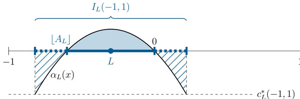
I illustrate the equilibrium outcome in Figure 4.19 Note that the challenger's equilibrium strategy described in Proposition 1 remains an equilibrium strategy of the public advertising game for a left-leaning non-baseline election with representative voter . See the proof of Theorem 1 for a full description of this equilibrium.
Swinging Elections with Targeted Advertising
In the remainder of this section, I focus on a baseline election that is unwinable with public advertising but winnable with targeted advertising. From Theorems 1 and 2, that election is polarized, so the unique decisive coalition that does not include a status quo voter is . The challenger wins if and only if left and right voters approve. Let us consider the following problem:
I will shortly show that this problem admits a solution such that is an interval with . Using the equilibrium construction from Theorem 2, I will conclude that the set is implementable; in the equilibrium that implements it, the challenger uses a direct strategy , his interim utility is and his odds of winning are .
Then, I will show that the pair also characterizes an optimal experiment that solves the information design problem, in which the challenger chooses and commits to an experiment prior to learning his policy outcome.20 Consequently, is the upper bound on the odds of convincing Bayesian voters and , and thus the highest odds of winning across all equilibria of the targeted advertising game. To understand why the challenger reaches this upper bound in an equilibrium of a verifiable information game, observe that Problem (AUX-TA) imposes only the voters' obedience constraints. Relative to an optimal experiment, an equilibrium strategy must satisfy additional incentive-compatibility constraints for the challenger (i.e., he must not have profitable deviations from an equilibrium strategy for each realized policy outcome ). However, given that his objective is to convince and to approve and that his messages must be verifiable, automatically satisfies these constraints; see the equilibrium construction in the proof of Theorem 2.
Let us now show that Problem (AUX-TA) admits a solution such that is a closed interval. For that, it is helpful to define the largest asymmetric interval of policy outcomes that each voter is willing to approve:
DEFINITION 5. The largest asymmetric interval of approved policy outcomes for voter is defined as follows:
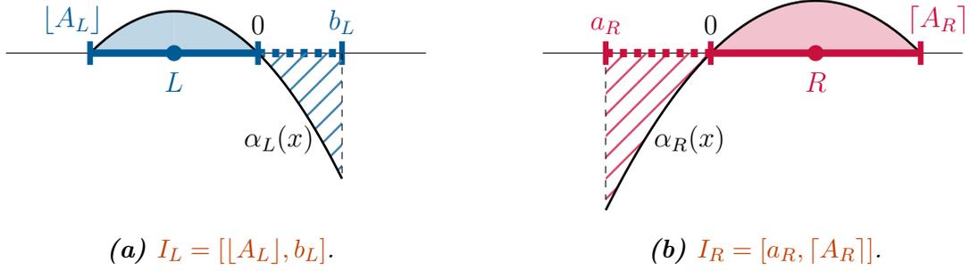
Simply put, includes 's approval set and as many right policy outcomes as her obedience constraint allows. Similarly, includes 's approval set and the largest set of left policy outcomes satisfying her obedience constraint. Figure 5 illustrates these intervals for quadratic voters and , and a uniform prior.21
One might guess that sending each voter her largest asymmetric interval—specifically, setting —maximizes the challenger’s odds of winning. This strategy is indeed optimal if , which occurs when and . It is straightforward to see that the challenger’s odds of winning cannot exceed : every policy outcome outside lies further from at least one voter’s bliss point, making it more “costly” in terms of that voter’s obedience constraint. Figure 6 illustrates this challenger-preferred equilibrium outcome for quadratic voters and , and a uniform prior.
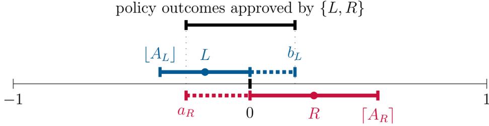
Next, consider the case when and . It is clear that sending each voter her largest asymmetric interval no longer maximizes the challenger’s odds of winning. Indeed, is now willing to approve ’s entire approval set as well as the policy outcomes left of , which left voters prefer to policy outcomes close to . Hence, should start at and span as far right as possible. Formally, in this case, and so that the challenger wins whenever .22 Figure 7 illustrates this outcome for quadratic voters , , and a uniform prior. The case when and is symmetric.
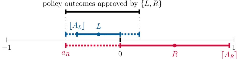
The final case, and , is impossible: these conditions would imply that voters and both prefer to approve under a common belief , contradicting (SC1).23 The following proposition summarizes the targeted advertising strategy that maximizes the challenger's odds of winning a polarized baseline election.
PROPOSITION 2. Consider a polarized baseline election, but . Then, the challenger's maximal odds of winning across all equilibria of the targeted advertising game are :
- If and , then
- If and , then
- If and , then
The challenger achieves these odds of winning by using the direct strategy .
The formal proof of this result is in the appendix and involves three steps. In step 1, I confirm that the pair solves Problem (AUX-TA). In step 2, I describe the equilibrium using the construction from the proof of Theorem 2. In step 3, I formulate the information design problem and show that the pair also characterizes an optimal experiment and the challenger's odds of winning are also .
Comparative Statics
Proposition 2 suggests that the boundaries of the challenger-preferred equilibrium set of winning policy outcomes depend on the voters' bliss points. I explore this relationship here. First, observe that more extreme voters are willing to approve wider ranges of policy outcomes.
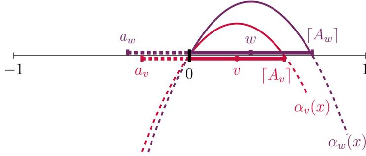
LEMMA 3. If is a more extreme voter than , then . Furthermore,
- if , then , and the inequality is strict if and ;
- if , then , and the inequality is strict if and .
Lemma 3 follows from the assumption (SC2) that more extreme voters are more persuadable. Figure 8 illustrates the intuition for Lemma 3 for right voters . First, observe that a more extreme voter would be persuaded by the most biased message intended for voter , that is, the interval is obedient for . Furthermore, a more extreme voter has a larger approval set (i.e., ), so the interval is obedient for also. Therefore, we can decrease the left boundary of that interval to so that the set remains obedient for ; the inequality is strict if and .
Next, let us explore how the challenger-preferred equilibrium outcome of a baseline election, described in Proposition 2, changes as right voters become more extreme. Note that making right voters more extreme makes the (already polarized) electorate more polarized (Esteban and Ray, 1994).
PROPOSITION 3. Consider the targeted advertising game with a polarized baseline election, but . Let be the challenger-preferred equilibrium intervals of approved policy outcomes described in Proposition 2. Suppose that . Then, as increases,
- the challenger's odds of winning increase;
- the set of winning policy outcomes shifts to the left, that is, and decrease.
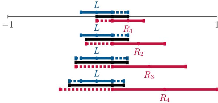
Figure 9 illustrates the equilibrium outcomes of four baseline elections, holding the left voters' bliss point fixed and increasing the right voters' bliss point from to (top to bottom).24 From Lemma 3, as right voters become more extreme, their largest asymmetric interval of approved policy outcomes expands. This has two consequences. First, these voters are now more persuadable, which means that the challenger's odds of winning go up. Second, more extreme right voters approve policy outcomes further to the left. As a result, the left boundary of the equilibrium set of winning policy outcomes shifts to the left, as well. Interestingly, the right endpoint of the equilibrium set of winning policy outcomes, which is determined by left voters, may strictly decrease, too. This happens when right voters are or become persuadable by policy outcomes left of (e.g., a change from to , or from to in Figure 9).
5. Discussion and Conclusion
This paper studied how a challenger advertises his privately known policy outcome to an electorate of voters with single-peaked and single-crossing preferences, using verifiable messages. Below I discuss how the analysis of the main model can be extended to other assumptions common in the political economy literature. I consider the following extensions: the presence of a strategic incumbent, a citizen-candidate challenger, probabilistic voting, instrumental voting, and information spillovers.
Strategic Incumbent
In the model, the incumbent does not advertise, and his policy outcome is known and normalized to zero. This assumption can be relaxed in a number of ways.
First, suppose that the status quo is a lottery, (independent of ), and the incumbent is still nonstrategic. Then, voter 's expected payoff from rejection is . While there are no left and right voters anymore (they were defined relative to 0), voters and can still be defined as having diametrically opposing preferences if implies for all , meaning that at most one of these voters prefers to approve given the choice between and any . Then, an election is unwinable for the challenger without targeted advertising if every decisive coalition requires convincing such voters. With targeted advertising, the challenger induces different posteriors among different voters and is still able to convince voters with diametrically opposing preferences with a positive probability.
Next, suppose that the incumbent is strategic and can change to a common belief about the status quo policy outcome, perhaps by publicly advertising it. Assuming that the challenger has time to react, he still benefits from targeted advertising for the same reason as in the above paragraph. In fact, even if the incumbent chooses the status quo policy outcome, the challenger can win as long as not every decisive coalition includes a status quo voter.
Finally, if the candidates are symmetric (e.g., they both use targeted advertising to advertise their own and/or their opponent's policy outcome), then full unraveling of information takes place (Janssen and Teteryatnikova, 2017; Schipper and Woo, 2019). Therefore, the key insight of this paper is that having access to better targeted-advertising technology and/or better voter data allows politicians to win otherwise unwinnable elections. Without this advantage, voters choose the same candidate as they would under complete information.
Citizen-candidate Challenger
In the main model, the challenger is office-motivated: his payoff is 1 if he wins and 0 if he loses. Let us consider an extension in which the challenger is a citizen-candidate whose payoff is if he wins and if he loses.25
It is easy to see that the equilibria described in Theorems 1 and 2 remain equilibria of the citizen-candidate games with public advertising and targeted advertising, respectively. In these equilibria, the challenger does not have profitable deviations when he wins because he reaches the highest possible payoff. On the other hand, he does not have profitable deviations when he loses due to voters' skeptical off-path beliefs, which ensure that he receives at most his complete information payoff if he deviates. Thus, as long as the challenger loses under complete information, whether his payoff depends on is irrelevant for the purpose of equilibrium construction.
Although the equilibria described in Propositions 1 and 2 maximize the challenger's odds of winning in a baseline election, they may not maximize his citizen-candidate ex-ante utility. It may be ex-ante optimal to let the set of winning policy outcomes include the most extreme challengers, as they would obtain the lowest payoff from losing. Characterizing the citizen-candidate's ex-ante optimal set of winning policy outcomes remains an open question.
Probabilistic Voting
In the model, the challenger knows the set of decisive coalitions. In this extension, I explore what happens if the challenger experiences uncertainty about which coalition is decisive. For concreteness, suppose that there are two possible voter bliss points, and , and the unique minimal decisive coalition is , , or with probability , , or , respectively. The timing of the game is the same, except the uncertainty about which coalition is decisive is resolved after the challenger chooses his messages.
It is useful to establish the challenger's payoff from fully revealing his policy outcome, as that provides the lower bound on his equilibrium payoff. Under full revelation (i.e., if the challenger's strategy is to send message for all ), his expected payoff is if , 1 if , and if . Furthermore, much like in the main model, deviations to full revelation are the only ones we need to rule out; other deviations can be made unprofitable by imposing voters' skeptical off-path beliefs. Below we analyze pure-strategy equilibria of public and targeted advertising games.
Public Advertising For any pure-strategy equilibrium, consider the mapping from the challenger's realized policy outcome to the actions taken by voters and . Since these voters never approve under a common belief, there are three possible outcomes for each : approves, approves, or no one approves. We can thus characterize a pure-strategy equilibrium outcome as a partition of the space of policy outcomes into those approved by the left coalition (), those approved by the right coalition (), and those approved by nobody (). Furthermore, we can implement any such partition by letting the challenger reveal which partition element his policy outcome belongs to: his partitional strategy is to send message if , message if , and message otherwise. For that to be an equilibrium strategy, must be obedient for voter . Moreover, the challenger must be obtaining at least his full revelation payoff.
One example of an equilibrium partitional strategy is “divide-and-conquer”—getting left (right) voters to approve the largest interval of left (right) policy outcomes (by letting and ). Another example of a partitional strategy is to maximize the odds of convincing the left voters (by letting and be the largest subset of obedient for ). In the end, the partitional strategy that maximizes the challenger’s odds of winning among pure-strategy equilibria will depend on parameters and .
Targeted Advertising It is easy to see that any direct strategy , where is obedient for voter and includes her approval set (e.g., the strategy described in Proposition 2), is an equilibrium strategy. The challenger’s ex-ante utility is then . It is also easy to see that, depending on the values of , and , letting —that is, maximizing the odds of convincing the mixed decisive coalition—may not maximize the challenger’s ex-ante utility. For example, if the left coalition is almost certainly decisive (), then tailoring the message to that coalition by letting increases the odds of winning.
Overall, when there is uncertainty about decisive coalitions, the challenger faces tradeoffs that are not present in the main model—in particular, he may want to cater to coalitions that are more likely to be decisive. The challenger-preferred equilibrium outcome characterization, whether the focus on pure-strategy equilibria is without loss, and whether the challenger reaches the same payoff as in information design, remain open questions.
Instrumental Voting
In the model, the voters have expressive preferences: if voter votes for policy outcome , then her payoff is . While this assumption is reasonable in large elections wherein the probability that an individual vote is pivotal is vanishingly small, in other elections voters may have instrumental concerns and derive utility also from the winning policy outcome. In this extension, I suppose that voters have both expressive (with probability ) and instrumental (with probability ) concerns. Suppose that voter 's payoff when she votes for policy outcome and the winning policy outcome is is . Below I argue that polarized elections remain winnable if and only if , that is, whenever the voters do not have purely instrumental concerns.
For concreteness, consider a polarized baseline election with voters and . For the same reasons as in the main model, the challenger-preferred equilibrium here is characterized by a pair of the voters' sets of approved policy outcomes obtained by solving26
Observe that the voters' obedience constraints now have two terms. The first term reflects the pivotality event, in which the winning policy outcome is because both voters approve. The second term is present only if the voters have expressive concerns (i.e., if ), as in that case, the winning policy outcome remains .
Suppose first that voters are purely instrumental, that is, . Then the obedience constraint of voter in the challenger-preferred equilibrium becomes . Crucially, that means that each voter's net payoff from approval is non-negative when she is pivotal, i.e., when both voters are recommended to approve. However, both voters are pivotal in the same event, whenever , and have a common posterior, , in that event. By (SC1), the unique common belief under which left and right voters prefer to approve is , so . Therefore, the challenger's odds of convincing purely instrumental and jointly pivotal voters and are zero even in his most-preferred equilibrium of the targeted advertising game.
If voters are not purely instrumental, that is, if , then there exists a pair that satisfies both voters' obedience constraints and .27 I thus conclude that polarized elections are winnable with targeted advertising even if there are only a small number of voters, as long as the voters' concerns are not purely instrumental.
Information Spillovers
The final key assumption of the model is that there are no information spillovers, meaning that the challenger's targeted ads stay private. If left and right voters observed each other's messages, they would learn the same information, making targeted advertising as good as public disclosure. Therefore, informing voters of all ads transmitted during an electoral campaign is a useful tool to mitigate the negative effects of targeted advertising. In fact, 1,433 targeted ads of the Vote Leave campaign were released in the aftermath of the 2016 Brexit referendum, but the release occurred after the vote was finalized.28
References
-
ALESINA, ALBERTO F. and RICHARD T. HOLDEN (2008), "Ambiguity and Extremism in Elections", June 2008, https://www.nber.org/papers/w14143, Working Paper.
-
ALONSO, RICARDO and ODILON CÂMARA (2016), "Persuading Voters", American Economic Review, 106, 11 (Nov. 2016), pp. 3590-3605.
-
ARAGONÈS, ENRIQUETA and ZVIKA NEEMAN (2000), "Strategic Ambiguity in Electoral Competition", Journal of Theoretical Politics, 12, 2 (Apr. 1, 2000), pp. 183-204.
-
ARIELI, ITAI and YAKOV BABICHENKO (2019), "Private Bayesian Persuasion", Journal of Economic Theory, 182 (July 2019), pp. 185-217.
-
ARTABE, ALAITZ and JAVIER GARDEAZABAL (2014), "Strategic Votes and Sincere Counterfactuals", Political Analysis, 22, 2 (Jan. 2014), pp. 243-257.
-
ASSEYER, ANDREAS and DILIP RAVINDRAN (2025), "Information Design with Competing Receivers", https://www.ssrn.com/abstract=5120732, Working Paper.
-
BAR-ISAAC, HESKI and JOYEE DEB (2014), “(Good and Bad) Reputation for a Servant of Two Masters”, American Economic Journal: Microeconomics, 6, 4 (Nov. 2014), pp. 293-325.
-
BARDHI, ARJADA and YINGNI GUO (2018), “Modes of Persuasion toward Unanimous Consent”, Theoretical Economics, 13, 3, pp. 1111-1149.
-
BERGEMANN, DIRK and STEPHEN MORRIS (2016), “Information Design, Bayesian Persuasion, and Bayes Correlated Equilibrium”, American Economic Review, 106, 5 (May 2016), pp. 586-591.
-
BRENNAN, GEOFFREY and LOREN LOMASKY (1993), Democracy and Decision: The Pure Theory of Electoral Preference, Cambridge University Press.
-
CALLANDER, STEVEN and CATHERINE H. WILSON (2008), “Context-Dependent Voting and Political Ambiguity”, Journal of Public Economics, 92 (Apr. 1, 2008).
-
CHAN, JIMMY, SEHER GUPTA, FEI LI, and YUN WANG (2019), “Pivotal Persuasion”, Journal of Economic Theory, 180 (Mar. 2019), pp. 178-202.
-
DRUCKMAN, JAMES N., MARTIN J. KIFER, and MICHAEL PARKIN (2009), “Campaign Communications in U.S. Congressional Elections”, American Political Science Review, 103, 3 (Aug. 2009), pp. 343-366.
-
ESTEBAN, JOAN-MARÍA and DEBRAJ RAY (1994), “On the Measurement of Polarization”, Econometrica, 62, 4, pp. 819-851.
-
FARRELL, JOSEPH and ROBERT GIBBONS (1989), “Cheap Talk with Two Audiences”, The American Economic Review, 79, 5, pp. 1214-1223.
-
FELSENTHAL, DAN S. and AVRAHAM BRICHTA (1985), “Sincere and Strategic Voters: An Israeli Study”, Political Behavior, 7, 4, pp. 311-324.
-
FOWLER, ERIKA FRANKLIN, MICHAEL M. FRANZ, GREGORY J. MARTIN, ZACHARY PESKOWITZ, and TRAVIS N. RIDOUT (2021), “Political Advertising Online and Offline”, American Political Science Review, 115, 1 (Feb. 2021), pp. 130-149.
-
GOLTSMAN, MARIA and GREGORY PAVLOV (2011), “How to Talk to Multiple Audiences”, Games and Economic Behavior, 72, 1 (May 1, 2011), pp. 100-122.
-
GROSSMAN, SANFORD J. (1981), “The Informational Role of Warranties and Private Disclosure about Product Quality”, The Journal of Law and Economics, 24, 3 (Dec. 1981), pp. 461-483.
-
GROSSMAN, SANFORD J. and OLIVER D. HART (1980), “Disclosure Laws and Takeover Bids”, The Journal of Finance, 35, 2, pp. 323-334.
-
HAMLIN, ALAN and COLIN JENNINGS (2011), “Expressive Political Behaviour: Foundations, Scope and Implications”, British Journal of Political Science, 41, 3 (July 2011), pp. 645-670.
-
HEESE, CARL and STEPHAN LAUERMANN (2025), “Persuasion and Information Aggregation in Elections”, Journal of Political Economy, 133, 10 (Oct. 2025), pp. 3305-3348.
-
HILLYGUS, D. SUNSHINE and TODD G. SHIELDS (2014), The Persuadable Voter: Wedge Issues in Presidential Campaigns, Princeton University Press, p. 267.
-
JANSSEN, MAARTEN C. W. and MARIYA TETERYATNIKOVA (2017), “Mystifying but not Misleading: when does Political Ambiguity not Confuse Voters?”, Public Choice, 172, 3-4 (Sept. 2017), pp. 501-524.
-
KAN, KAMHON and C. C. YANG (2001), “On Expressive Voting: Evidence from the 1988 U.S. Presidential Election”, Public Choice, 108, 3-4, pp. 295-312.
-
KARTIK, NAVIN, SANGMOK LEE, and DANIEL RAPPOPORT (2024), “Single-Crossing Differences in Convex Environments”, The Review of Economic Studies, 91, 5 (Oct. 2024), pp. 2981-3012.
-
KARTIK, NAVIN, RICHARD VAN WEELDEN, and STEPHANE WOLTON (2017), “Electoral Ambiguity and Political Representation”, American Journal of Political Science, 61, 4, pp. 958-970.
-
KENDALL, CHAD, TOMMASO NANNICINI, and FRANCESCO TREBBI (2015), “How Do Voters Respond to Information? Evidence from a Randomized Campaign”, American Economic Review, 105, 1 (Jan. 2015), pp. 322-353.
-
KOEGLER, FRÉDÉRIC (2008), “Lobbying with Two Audiences: Public vs Private Certification”, Mathematical Social Sciences, 55, 3 (May 1, 2008), pp. 305-314.
-
KOLOTILIN, ANTON, TYMOFIY MYLOVANOV, ANDRIY ZAPACHELNYUK, and MING LI (2017), “Persuasion of a Privately Informed Receiver”, Econometrica, 85, 6, pp. 1949-1964.
-
LE PENNEC, CAROLINE and VINCENT PONS (2023), “How do Campaigns Shape Vote Choice? Multicountry Evidence from 62 Elections and 56 TV Debates”, The Quarterly Journal of Economics, 138, 2 (May 1, 2023), pp. 703-767.
-
MEIROWITZ, ADAM (2005), “Informational Party Primaries and Strategic Ambiguity”, Journal of Theoretical Politics, 17, 1 (Jan. 1, 2005), pp. 107-136.
-
MILGROM, PAUL R. (1981), “Good News and Bad News: Representation Theorems and Applications”, The Bell Journal of Economics, 12, 2, p. 380.
-
PAGE, BENJAMIN I (1978), Choices and Echoes in Presidential Elections: Rational Man and Electoral Democracy, University of Chicago Press.
-
PERSSON, TORSTEN and GUIDO TABELLINI (2002), Political Economics: Explaining Economic Policy, The MIT Press.
-
SCHIPPER, BURKHARD C. and HEE YEUL WOO (2019), “Political Awareness, Microtargeting of Voters, and Negative Electoral Campaigning”, Quarterly Journal of Political Science, 14, 1 (Jan. 10, 2019), pp. 41-88.
-
SCHNAKENBERG, KEITH E. (2015), “Expert Advice to a Voting Body”, Journal of Economic Theory, 160 (Dec. 1, 2015), pp. 102-113.
-
SHEPSLE, KENNETH A. (1972), “The Strategy of Ambiguity: Uncertainty and Electoral Competition”, American Political Science Review, 66, 2 (June 1972), pp. 555-568.
-
SPENKUCH, JÖRG L and DAVID TONIATTI (2018), “Political Advertising and Election Results”, The Quarterly Journal of Economics, 133, 4 (Nov. 1, 2018), pp. 1981-2036.
-
TITOVA, MARIA and KUN ZHANG (2025), “Persuasion with Verifiable Information”, Journal of Economic Theory, 230 (Dec. 1, 2025), p. 106102.
-
TOLVANEN, JUHA (2024), “On Political Ambiguity and Anti-Median Platforms”, European Economic Review, 170 (Nov. 1, 2024), p. 104884.
Appendix
LEMMA A.1. Let and suppose that voter is more extreme than . Then:
Proof. By (SC2), for all , so . Next, write as a partition into disjoint sets and . Therefore,
where the last term is non-negative because for all . Consequently, implies (by SC2), which implies . ■
Proof of Lemma 2
If , then solves Problem (AUX). We thus assume for the remainder of the proof that .
We first show that the set is well-defined. Since is strictly quasiconcave, the set is convex (i.e., is an empty set, a point, or a closed interval) for any . Furthermore, expands as decreases, i.e., if , then ; the inclusion is strict unless . Now, let . By the dominated convergence theorem, is continuous ( is continuous and bounded, while is a finite measure). Observe that since ; here, because .
Next, let ; note that if and only if and thus . Observe that is strictly increasing in for . Indeed, if , then
since for all and if . By the intermediate value theorem, there exists a unique such that .
We now show that all solutions to Problem (AUX) agree with -almost everywhere. Let be an arbitrary solution. The obedience constraint binds for and holds for , therefore:
Now, since , we have for all and . We thus obtain:
since ; these inequalities are strict unless . Therefore, is a solution if and only if it agrees with -almost everywhere.
LEMMA A.2. Let be the interval solution to Problem (AUX) for voter with and . Suppose that . Let and be the unique solution to . Then:
- and if ;
- and if ;
- and if .
Proof. Note that we showed the existence of in the proof of Lemma 2. Also note that . Furthermore, recall that ; since , it follows that . Consequently, if (as in cases 1 and 2), then , (since is strictly increasing on ) and thus from cases 1 and 2 is well-defined. We have:
- If , let and solve .29 Then, as desired.
- If , let solve so that .
- If , let solve so that . ■
LEMMA A.3. Let . Also, let and be the interval solutions to Problem (AUX) for voter with (resp.) and . Then, and .
Proof. Observe that implies . Therefore, if , then and , and the claim is true. For the rest of the proof, assume . Let and be the unique solution to . Also, let be the unique solution to if it exists (i.e., if ). From Lemma A.2, we have three possible cases:
- so that , and :
- (i) , so , , and thus .
- (ii) . If , then and the claim holds since and . Else, if , then exists, and:
so that since the function is strictly increasing in (see the proof of Lemma 2). Therefore, we have
and by Lemma A.2 (case 3), , where , and the claim holds.
- so that , and . Then, if , we have so that . If, on the other hand, , then , so , , and thus . Overall, in case 2 we have and the claim holds.
- If , then , , and . If , then and the claim holds. If , then by the same argument as in case 1.(ii). Consequently, by Lemma A.2 (case 3), , where . Overall, in case 3 we have , where , , and the claim holds. ■
Proof of Proposition 2
Step 1: Show that Problem (AUX-TA) admits a solution
- and if and ;
- and if and ;
- and if and .
Suppose that such that for each is an arbitrary solution to Problem (AUX-TA).30 Let , , and:
We will use the voters' obedience constraints to show that , which implies that is a solution to Problem (AUX-TA). By contradiction, suppose that . We will address cases 1 and 2 (each with multiple subcases), in which ; case 3 is proved analogously to case 2.
1.1 and . In this case, ; also, , , , and . First, note that binds 's obedience constraint since , we have and . Similarly, binds 's obedience constraint since .
Then, we can partition31 into three sets , and , and write down 's (binding) obedience constraint for as:
Similarly, we partition into four sets , , and , and write down 's obedience constraint for as:
where the last inequality holds because (so that and ) and is negative outside . Combining (1) and (2), we get:
Since , , and is strictly decreasing on , we get:
which implies that since . Using the same argument (i.e., by comparing the terms in 's obedience constraints for and ), we obtain . Therefore, , a contradiction.
1.2 and . In this case, 's constraint for is binding (since ), while 's constraint for may or may not bind.
Using the fact that binds 's constraint, we obtain (see step 1.1). While 's constraint for may not bind, from we have and , so and . Therefore, , a contradiction.
1.3 and . This case is analogous to 1.2.
1.4 and . This case is impossible because then for each , i.e., both voters weakly prefer to approve under the prior ; that contradicts (SC1).
2.1 and . In this case, and .32 Since solves Problem (AUX) with and for voter , which is Problem (AUX-TA) without 's obedience constraint, the pair also solves (AUX-TA).
2.2 and . In this case, , and . Also, , , , and . It is worth mentioning that and are different objects: is the upper bound of , while is the upper bound of . By Lemma A.3, we have . Now, since , we have , so and 's constraint for binds. From that, (see step 1.1).
For voter , two cases are possible: and . If , then satisfies and 's obedience constraints, i.e., both voters prefer to approve under belief , which contradicts (SC1). Therefore, .
Now, we have and , i.e., binds 's obedience constraint. Partition into , , , , , and write down 's (binding) obedience constraint for as:
Similarly, partition into , , , , . Using the fact that and is negative outside , from the obedience constraint for we obtain
Combining (3) and (4), we get
and, since for all , and for all , , we obtain
since .
Next, observe that if , then . Indeed, since and , from Lemma 2 we get that for some . In particular, we have for all and for all , which is a non-empty set if . By the continuity and strict monotonicity of on , we have so that .
Now, dividing the last inequality by , we get:
Next, add to both sides to obtain:
Rearranging terms, we get:
since if and from the previous calculations in the beginning of step 2.2. Therefore, , a contradiction.
3 and . This case is analogous to case 2.
Step 2: Equilibrium Characterization.
Observe that the mixed decisive coalition is ; the set is an interval such that and ; the set satisfies the obedience constraint of voter . Thus, is implementable and the equilibrium that implements is described in the proof of Theorem 2; the equilibrium strategy of the challenger is
Step 3: Show that there exists an optimal experiment that is characterized by , for which the challenger's odds of winning are .
The challenger's information design problem is formulated as follows.33 First, the challenger chooses and commits to an experiment, which is a measurable map . Next, the challenger's policy outcome is realized according to and the signals and are sent to voters with bliss points and (resp.) with probability . Then, voter privately observes her signal , forms a posterior belief using the Bayes rule, and approves after and rejects after . Let be the marginal probability that receives signal . For to approve after signal , her net payoff from approval must be non-negative:
Similarly, for to reject after signal , her expected net payoff from approval must be negative, . An optimal experiment maximizes the challenger's odds of winning and solves
Moreover, we can drop the less-than-zero constraints as letting for each and weakly increases the objective and loosens 's constraints. Now, since each is bounded, is a finite and atomless positive measure, and is a closed interval, a deterministic optimal experiment exists (by an argument similar to one in the proof of Proposition 2 in Titova and Zhang, 2025). Next, let for each be the set of policy outcomes that is recommended to approve. Then, an optimal deterministic experiment is characterized by a pair that solves Problem (AUX-TA). Hence, is the challenger's odds of winning in the information design problem.
Proof of Lemma 3
We prove this statement for left voters . The proof for right voters is analogous. From the definition of () as a solution to Problem (AUX) with () and , three cases are possible:
Case 1 . Then, . By (SC2), so and since .
Case 2 and . Then, , where and . Therefore, .
Case 3 and . Then, , where and ; the same is true for —in particular, . By (SC2), (the last inequality is strict unless ). Now, since the function is continuous and strictly decreasing in for , we have
so that . Furthermore, unless , we have and .
Proof of Proposition 3
Let be the baseline electorate with the more extreme right voter . Let be the solution to (AUX-TA) for this electorate (described in Proposition 2). Note that and imply that , so and are both described by Case 1 or 2 of Proposition 2. Therefore, , and, by Lemma 3, . To simplify exposition, let and .
If , then both elections fall into case 1 of Proposition 2. We have , , and the claims of the proposition are true because .
Next, suppose that , in which case . Observe that is decreasing in (which is a parameter in Problem AUX) on : increasing shrinks the feasible region , so the objective value can only go down. Therefore, for all . In particular, if , then , and if , then . Either way, .
Finally, from Lemma A.3, both boundaries of are left of the corresponding boundaries of (often strictly so—see the proof of Lemma A.3). If , then and so is left of . If, on the other hand, , then is left of , which is a superset of , so is left of .